Bernoulli Multi-Armed Bandit Problem

Abstract

A practical introduction to the exploration-exploitation trade-off through epsilon-greedy, upper confidence bounds, and Thompson Sampling on Bernoulli bandits.

Note

This post builds on Lilian Weng’s overview. I worked through the derivations and implementations to clarify the statistical ideas for myself.

The exploration-exploitation trade-off appears whenever a familiar option offers a predictable result but an unfamiliar option might be better. Always choosing the familiar option prevents discovery; always trying something new produces avoidable disappointments.

A multi-armed bandit isolates this trade-off. The goal is to collect as much reward as possible while learning which actions are valuable. Exploitation uses current estimates, while exploration accepts a possible short-term loss to improve those estimates.

This is also a minimal reinforcement learning setting: one state, a discrete set of actions, and immediate rewards without state transitions. I use it to compare four strategies: \(\epsilon\)-greedy, a UCB1-style rule, a Bayesian UCB-style heuristic, and Thompson Sampling.

What Is a Multi-Armed Bandit?

The multi-armed bandit (MAB) models a row of slot machines, or one-armed bandits, each with an unknown payout probability. The goal is to maximize total reward over time. Every pull provides information, but it also uses a trial that could have gone to a better machine.

The Environment

Consider several slot machines, each with an unknown Bernoulli reward distribution. A play returns either \(1\) or \(0\). You have a fixed number of trials \(T\), and your choices do not change the underlying probabilities. The problem is to choose actions that produce high reward while revealing enough information to improve later choices.

Note

Regret measures the expected reward lost by choosing an arm other than the one with the highest reward probability.

The solver does not know the reward probabilities. It must estimate them through interaction.

from abc import ABC, abstractmethod
from pathlib import Path

import matplotlib.pyplot as plt
import numpy as np
import numpy.typing as npt
from aquarel import load_theme
from matplotlib.figure import Figure
from scipy.stats import beta

DPI = 200  # 2x the ~800px content column, so figures stay crisp on HiDPI screens
FIGURES = Path("./figures")


def save_fig(fig: Figure, name: str) -> None:
    """Write a figure into figures/ as lossless WebP, keeping the transparent background."""
    FIGURES.mkdir(parents=True, exist_ok=True)
    fig.savefig(FIGURES / name, dpi=DPI, transparent=True, pil_kwargs={"lossless": True, "method": 6})
    plt.close(fig)

class BaseBandit(ABC):
    k: int  # number of arms
    best_proba: float | np.float64  # hidden to solver; for regret calculation, highest possible reward probability
    probas: npt.NDArray[np.float64]  # hidden to solver; reward probabilities

    @abstractmethod
    def generate_reward(self, i: int) -> float:
        """Returns reward after lever `i` is pulled."""
        raise NotImplementedError


class BaseSolver(ABC):
    bandit: BaseBandit  # reference to the bandit instance
    counts: npt.NDArray[np.int64]  # hold stats of pulled levers

    actions: list[int]
    rewards: list[float]
    regrets: list[float]

    @abstractmethod
    def __init__(self, bandit: BaseBandit) -> None:
        """bandit (BaseBandit): the target bandit to solve."""
        assert isinstance(bandit, BaseBandit)
        self.bandit = bandit

        self.counts = np.zeros(self.bandit.k, dtype=np.int64)

        self.actions = []  # a history of lever ids, 0 to bandit n-1.
        self.rewards = []  # a history of collected rewards.
        self.regrets = []  # a history of regrets for taken actions.

    @property
    def num_steps(self) -> int:
        return len(self.actions)

    def update_regret(self, i: int) -> None:
        """Update the regret after the lever `i` is pulled."""
        regret = self.bandit.best_proba - self.bandit.probas[i]
        self.regrets.append(regret)

    @property
    @abstractmethod
    def estimated_probas(self) -> npt.NDArray[np.float64]:
        """Retrieve learned reward probability for each arm `n` of the bandit."""
        raise NotImplementedError

    @abstractmethod
    def run_one_step(self) -> tuple[int, float]:
        """Return solver's selected action and bandit's outcome reward."""
        raise NotImplementedError

    def run(self, num_steps: int) -> None:
        """Run simulation for `num_steps` steps."""
        for _ in range(num_steps):
            i, r = self.run_one_step()

            self.counts[i] += 1
            self.actions.append(i)
            self.update_regret(i)
            self.rewards.append(r)

Formal Definition

A Bernoulli bandit is a tuple \(\langle \mathcal{A}, \mathcal{R} \rangle\):

• There are \(K\) machines, or arms, with reward probabilities \(\{\theta_1, \ldots, \theta_K\}\).
• At time step \(t\), the solver selects action \(a_t\) and receives reward \(r_t\).
• \(\mathcal{A}\) is the set of possible actions. An action’s value is its expected reward, \(Q(a) = \mathbb{E}[r \mid a]\). If \(a_t\) selects arm \(i\), then \(Q(a_t) = \theta_i\).
• \(\mathcal{R}\) is the reward function. In a Bernoulli bandit, a pull returns \(1\) with probability \(Q(a_t)\) and \(0\) otherwise.

Note

A Bernoulli distribution takes the value \(1\) with probability \(p\) and \(0\) with probability \(1-p\).

The symbol \(\mathbb{E}[\cdot]\) denotes expected value, a probability-weighted average. The expression \(\mathbb{E}[r \mid a]\) means the expected reward conditional on taking action \(a\).

The probabilities \(\{\theta_i\}\) are unknown to the solver and must be estimated through interaction.

A Bernoulli bandit is a simplified Markov decision process without state transitions. Maximizing total reward, \(\sum_{t=1}^{T} r_t\), is equivalent in expectation to minimizing regret relative to the optimal arm.

Let \(\theta^*\) denote the reward probability of the optimal action \(a^*\):

\[ \theta^* = Q(a^*) = \max_{a \in \mathcal{A}} Q(a) = \max_{1 \leq i \leq K} \theta_i. \]

The expected cumulative regret through time \(T\) is

\[ \mathcal{L}_T = \mathbb{E}\left[\sum_{t=1}^{T}\left(\theta^* - Q(a_t)\right)\right]. \]

class BernoulliBandit(BaseBandit):
    def __init__(
        self,
        k: int,
        probas: list[float] | npt.NDArray[np.float64] | None = None,
        seed: int | None = None,
    ):
        # sanity check: `probas` needs to be None or of size `n`.
        assert probas is None or len(probas) == k

        self.k = k  # save number of bandits

        self.rng = np.random.default_rng(seed=seed)

        # random probabilities, if they are explicitly defined
        if probas is None:
            probas = self.rng.random(size=self.k)

        # convert to numpy array for easier operations later
        self.probas = np.asarray(probas)

        # in case of Bernoulli MAB, highest probability is equal to optimal
        self.best_proba = np.max(self.probas)

    def generate_reward(self, i: int) -> float:
        # The player selected the i-th machine.
        return float(self.rng.random() < self.probas[i])

Bandit Strategies

Bandit strategies differ mainly in how they gather information:

• Greedy selection uses only the best current estimate and does not explore deliberately.
• Random exploration sometimes ignores the estimates and selects an arm at random.
• Informed exploration directs trials toward arms whose values remain uncertain.

The \(\epsilon\)-greedy algorithm is the simplest random-exploration strategy.

Epsilon-Greedy Algorithm

The \(\epsilon\)-greedy algorithm balances exploitation and exploration by choosing the currently best action most of the time, while occasionally exploring at random.

Information State

At time step \(t\), the algorithm maintains:

• empirical action-value estimates \(\hat{Q}_t(a)\),
• action counts \(N_t(a)\),

summarizing all past interactions.

The empirical value estimate for action \(a\) is defined as:

\[ \hat{Q}_t(a) = \frac{1}{N_t(a)} \sum_{\tau = 1}^t r_\tau \cdot \mathbb{1}[a_\tau = a] \]

where:

• \(r_\tau\) is the reward received at time step \(\tau\). For a Bernoulli bandit, this is either \(1\) (success) or \(0\) (no reward).
• \(\mathbb{1}[a_\tau = a]\) is an indicator function equal to \(1\) when action \(a\) was taken at time \(\tau\), and \(0\) otherwise.
• \(N_t(a)\) is the number of times action \(a\) has been selected: \[ N_{t}(a) = \sum_{\tau = 1}^t \mathbb{1}[a_\tau = a] \]

Policy

The \(\epsilon\)-greedy policy defines a stochastic action-selection rule:

• with probability \(1 - \epsilon\), the greedy action is selected: \[ \hat{a}^{*}_t = \arg\max_{a\in\mathcal{A}} \hat{Q}_t(a) \]
• with probability \(\epsilon\), an action is selected uniformly at random.

Equivalently, the policy can be written as:

\[ \pi(a|h_t) = \begin{cases} 1 - \epsilon + \frac{\epsilon}{|\mathcal{A}|}, & a = a^*_t, \\ \frac{\epsilon}{|\mathcal{A}|}, & \text{otherwise}. \end{cases} \]

Update Rule

After selecting action \(a_t\) and observing reward \(r_t\), the estimate \(\hat{Q}_t(a_t)\) is updated using the new observation.

Note

Despite its simplicity, \(\epsilon\)-greedy often performs reasonably well. However, because exploration is random and does not depend on uncertainty, it can waste trials on clearly suboptimal actions.

class EpsilonGreedy(BaseSolver):
    def __init__(self, bandit: BaseBandit, eps: float, init_proba: float = 1.0, seed: int | None = None) -> None:
        """
        eps (float): the probability to explore at each time step.
        init_proba (float): default to be 1.0; optimistic initialization
        """
        super().__init__(bandit)

        assert 0.0 <= eps <= 1.0
        self.eps = eps

        # optimistic initialization
        self.estimates = np.full(self.bandit.k, fill_value=init_proba, dtype=np.float64)

        # define random generator with seed for reproducibility
        self.rng = np.random.default_rng(seed=seed)

    @property
    def estimated_probas(self) -> npt.NDArray[np.float64]:
        return self.estimates

    def run_one_step(self) -> tuple[int, float]:
        # With probability epsilon pick random exploration, or pick the known best lever.

        if self.rng.random() < self.eps:
            # pure random exploration
            i = int(self.rng.integers(0, self.bandit.k))
        else:
            # greedy selection with random tie-breaking
            candidates = np.flatnonzero(self.estimates == self.estimates.max())
            i = int(self.rng.choice(candidates))

        r = self.bandit.generate_reward(i)
        self.estimates[i] += 1.0 / (self.counts[i] + 1) * (r - self.estimates[i])

        return i, r

Upper Confidence Bounds

Random exploration can waste trials on actions that are already known to be poor. Two alternatives are to decay \(\epsilon\) over time or to favor actions whose estimates remain uncertain. The second approach leads to upper confidence bound (UCB) algorithms.

A UCB method assigns each action an optimistic score,

\[ \hat{Q}_t(a) + \hat{U}_t(a), \]

where \(\hat{Q}_t(a)\) is the empirical reward estimate and \(\hat{U}_t(a)\) is an uncertainty bonus. With high probability, the score should exceed the true value:

\[ Q(a) \leq \hat{Q}_t(a) + \hat{U}_t(a). \]

The bonus shrinks as \(N_t(a)\), the number of pulls of action \(a\), grows. Selecting the largest score therefore balances high estimated reward against limited evidence.

Unified Definition

Information State

At time step \(t\), a UCB algorithm maintains:

• empirical action-value estimates \(\hat{Q}_t(a)\),
• action counts \(N_t(a)\).

These quantities summarize the full interaction history.

Policy

Ignoring tie-breaking, UCB defines a deterministic policy:

\[ \pi(a|h_t) = \begin{cases} 1, & a = \arg\max_{a'} \left[ \hat{Q}_t(a') + \hat{U}_t(a') \right], \\ 0, & \text{otherwise}. \end{cases} \]

Unlike \(\epsilon\)-greedy, exploration is not injected explicitly. Instead, it emerges through optimism in the face of uncertainty.

Action Selection

At each time step, the selected action is:

\[ a_t = \arg\max_{a \in \mathcal{A}} \left[ \hat{Q}_t(a) + \hat{U}_t(a) \right]. \]

Update Rule

After selecting action \(a_t\) and observing reward \(r_t\), the algorithm updates:

• the action counts \(N_t(a_t)\)
• the empirical estimate \(\hat{Q}_t(a_t)\)

Choosing the Uncertainty Bound

The remaining design choice is how to define \(\hat{U}_t(a)\). Different choices lead to different members of the UCB family, such as UCB1, which derives its bound from Hoeffding’s inequality.

Hoeffding’s Inequality

If we do not want to assign any prior knowledge about the shape of the reward distribution (e.g., Gaussian, exponential), we can rely on Hoeffding’s Inequality. This theorem is applicable on any bounded distribution.

A random variable is said to follow a bounded distribution if all its values lie within a fixed finite interval \([a,b]\). In our case, Bernoulli rewards always lie in \([0,1]\), so the boundedness assumption is naturally satisfied.

Note

Here are a few examples for intuition:

• A Bernoulli distribution is bounded on interval \([0,1]\).
• A uniform distribution on interval e.g., \([2,5]\) is bounded.
• A Gaussian distribution is not bounded because of its infinite tails.

Hoeffding’s Inequality (Informal Version)

Let \(X_1, \ldots, X_t\) be i.i.d. (independent and identically distributed) random variables, all bounded in the interval \([0,1]\). The sample mean is

\[ \overline{X}_t = \frac{1}{t} \sum_{\tau = 1}^{t} X_{\tau}. \]

Then for any \(u \gt 0\), Hoeffding’s inequality states:

\[ \mathbb{P}\left[\mathbb{E}[X] \gt \overline{X}_{t} + u \right] \leq \mathrm{e}^{-2tu^2}. \]

This inequality bounds the probability that the true mean exceeds the empirical mean by more than \(u\).

Applying Hoeffding’s Inequality to Bandit Rewards

To apply this result to the multi-armed bandit setting, we observe that each fixed action \(a\) defines its own random reward-generating process. Every time we select action \(a\), we obtain a reward drawn independently from the same bounded distribution. Therefore, Hoeffding’s inequality applies directly to each arm.

For a fixed target action \(a\), define:

• \(r_{\tau}(a)\) as the reward random variable,
• \(Q(a)\) as the true mean reward,
• \(\hat{Q}_{t}(a)\) as the sample mean reward,
• and \(u = U_{t}(a)\) as the upper confidence bound.

By directly identifying Hoeffding’s variables with the bandit quantities:

\[ X_{\tau} \leftrightarrow r_\tau(a),\quad \mathbb{E}[X] \leftrightarrow Q(a),\quad \overline{X} \leftrightarrow \hat{Q}_{t}(a),\quad t \leftrightarrow N_{t}(a) \]

we obtain:

\[ \mathbb{P} \left[ Q(a) \gt \hat{Q}_{t}(a) + U_{t}(a) \right] \leq \mathrm{e}^{-2 N_{t}(a) U_{t}(a)^2}. \]

This gives a probabilistic upper bound on how much the true reward of an action can exceed its empirical estimate.

Choosing the Upper Confidence Bound

We want to select the confidence bound so that the probability of underestimating the true mean is very small. Let us require this probability to be below a small threshold \(p\):

\[ \mathrm{e}^{-2N_{t}(a)U_{t}(a)^2} = p. \]

Solving for \(U_{t}(a)\), we obtain:

\[ U_{t}(a) = \sqrt{\frac{-\ln{p}}{2N_{t}(a)}}. \]

This expression defines how much optimism we should add to the empirical estimate based on how many times the action has been sampled.

UCB1

For rewards bounded in \([0,1]\), Hoeffding’s inequality gives the confidence radius

\[ U_t(a) = \sqrt{\frac{-\ln p}{2N_t(a)}}. \]

Choosing \(p=t^{-4}\) gives

\[ U_t(a) = \sqrt{\frac{2\ln t}{N_t(a)}}. \]

The classic UCB1 rule first pulls every arm, then selects (Auer et al. 2002)

\[ a_t^{\textrm{UCB1}} = \arg\max_{a \in \mathcal{A}}\left[\hat{Q}_t(a) + \sqrt{\frac{2\ln t}{N_t(a)}}\right]. \]

The empirical estimate \(\hat{Q}_t(a)\) favors exploitation. The square-root term favors arms with fewer observations, while \(\ln t\) lets the bonus for a neglected arm grow as time passes.

Note

The class below is a UCB1-style variant. It initializes every estimate to \(1\), uses \(1+N_t(a)\) in the denominator, and does not force one initial pull per arm. The benchmark retains the label “UCB1” as shorthand for this implementation.

class UCB1(BaseSolver):
    def __init__(self, bandit: BaseBandit, init_proba: float = 1.0, seed: int | None = None):
        super().__init__(bandit)
        self.t = 0  # number of time steps
        self.estimates = np.full(shape=self.bandit.k, fill_value=init_proba, dtype=np.float64)
        self.rng = np.random.default_rng(seed)

    @property
    def estimated_probas(self) -> npt.NDArray[np.float64]:
        return self.estimates

    def run_one_step(self) -> tuple[int, float]:
        self.t += 1

        # Pick the best one with consideration of upper confidence bounds.
        ucb = self.estimates + np.sqrt(2 * np.log(self.t) / (1 + self.counts))

        # tie-breaking
        candidates = np.flatnonzero(ucb == ucb.max())
        i = int(self.rng.choice(candidates))

        r = self.bandit.generate_reward(i)

        self.estimates[i] += 1.0 / (self.counts[i] + 1) * (r - self.estimates[i])

        return i, r

Beta-Posterior UCB Heuristic

A Bayesian bandit maintains a posterior distribution for each arm’s unknown reward probability. Formal Bayes-UCB selects an upper posterior quantile whose level changes with time (Kaufmann et al. 2012).

The implementation below uses a related but simpler rule for Bernoulli rewards. Each arm has a Beta posterior,

\[ \theta_a \mid h_t \sim \textrm{Beta}(\alpha_a, \beta_a), \]

with posterior mean and standard deviation

\[ \mu_t(a) = \frac{\alpha_a}{\alpha_a + \beta_a}, \qquad \sigma_t(a) = \operatorname{std}\!\left[\textrm{Beta}(\alpha_a, \beta_a)\right]. \]

After pulling every arm once, the solver selects

\[ a_t = \arg\max_{a \in \mathcal{A}}\left[\mu_t(a) + c\sigma_t(a)\right]. \]

The mean favors arms that currently look rewarding, while the standard-deviation bonus favors uncertain arms. A Beta\((1,1)\) prior initializes every arm uniformly, and the default \(c=2\) controls the size of the uncertainty bonus.

This mean-plus-standard-deviation score is a heuristic, not the formal posterior-quantile Bayes-UCB algorithm. For a Gaussian posterior it would correspond to a fixed quantile, but a finite-sample Beta posterior is generally asymmetric. The class and figure use “Bayesian UCB” as a short label for the implemented heuristic.

Comparison with UCB1

Method	Estimate	Exploration bonus
UCB1-style implementation	Empirical mean	Count-based Hoeffding-style bonus
Implemented Bayesian UCB-style heuristic	Beta posterior mean	\(c\) times the Beta posterior standard deviation
Formal Bayes-UCB	Posterior distribution	Time-dependent posterior quantile

class BayesianUCB(BaseSolver):
    def __init__(
        self,
        bandit: BaseBandit,
        c: float = 2,
        init_a: float = 1,
        init_b: float = 1,
        deterministic: bool = True,
        seed: int | None = None,
    ) -> None:
        super().__init__(bandit)

        self.c = c
        self._as = np.full(self.bandit.k, fill_value=init_a, dtype=np.float64)
        self._bs = np.full(self.bandit.k, fill_value=init_b, dtype=np.float64)

        self.t = 0

        self.is_deterministic = deterministic
        self.rng = np.random.default_rng(seed)

    @property
    def estimated_probas(self) -> npt.NDArray[np.float64]:
        return self._as / (self._as + self._bs)

    def run_one_step(self) -> tuple[int, float]:

        self.t += 1

        # ensure each arm is tried at least once
        if self.t <= self.bandit.k:
            i = self.t - 1
        else:
            mu = self._as / (self._as + self._bs)  # posterior mean
            sigma = beta.std(self._as, self._bs)  # posterior std Beta(alpha, beta)
            confidence = mu + self.c * sigma

            # tie-breaking in case of two or more equal confidence weights
            if self.is_deterministic:
                # tie-breaking by lowest index (deterministic)
                i = int(np.argmax(confidence))
            else:
                # tie-breaking by random pick (non-deterministic)
                candidates = np.flatnonzero(confidence == confidence.max())
                i = int(self.rng.choice(candidates))

        r = self.bandit.generate_reward(i)

        # update Beta posterior for Bernoulli reward
        self._as[i] += r  # successes
        self._bs[i] += 1 - r  # failures

        return i, r

Thompson Sampling

Thompson Sampling is a probability-matching policy: it selects an action according to its posterior probability of being optimal (Thompson 1933). Instead of constructing an upper bound, it samples one plausible reward probability for every arm and chooses the largest sample.

At each time step, the solver:

1. Samples one reward probability from each arm’s posterior.
2. Selects the arm with the largest sample.
3. Observes the reward and updates that arm’s posterior.

Uncertain arms have wider posteriors and can occasionally produce large samples, which drives exploration. Arms with high posterior means produce large samples more consistently, which drives exploitation.

Thompson Sampling for Bernoulli Bandits

For a Bernoulli bandit, the conjugate prior is the Beta distribution:

\[ \theta_a \sim \textrm{Beta}(\alpha_a, \beta_a). \]

A Beta\((1,1)\) prior is uniform over \([0,1]\). After observing reward \(r_t \in \{0,1\}\) from the selected arm, the posterior update is

\[ \alpha_a \leftarrow \alpha_a + r_t, \qquad \beta_a \leftarrow \beta_a + (1-r_t). \]

The action rule samples

\[ \widetilde{\theta}_a \sim \textrm{Beta}(\alpha_a, \beta_a) \quad \textrm{for every } a \in \mathcal{A}, \]

then selects

\[ a_t^{\textrm{TS}} = \arg\max_{a \in \mathcal{A}} \widetilde{\theta}_a. \]

This is exact posterior updating for the Beta-Bernoulli model.

Relationship to Bayesian UCB

Formal Bayes-UCB acts on a time-dependent upper posterior quantile. The heuristic in this notebook acts on the posterior mean plus \(c\) standard deviations. Thompson Sampling draws directly from each posterior. All three use uncertainty, but they turn it into actions differently: an upper quantile, a scale bonus, or a random posterior sample.

class ThompsonSampling(BaseSolver):
    def __init__(self, bandit: BaseBandit, init_a: int = 1, init_b: int = 1, seed: int | None = None) -> None:
        super().__init__(bandit)

        self._as = np.full(self.bandit.k, fill_value=init_a, dtype=np.float64)
        self._bs = np.full(self.bandit.k, fill_value=init_b, dtype=np.float64)

        self.rng = np.random.default_rng(seed)

    @property
    def estimated_probas(self) -> npt.NDArray[np.float64]:
        return self._as / (self._as + self._bs)

    def run_one_step(self) -> tuple[int, float]:
        samples = self.rng.beta(self._as, self._bs)

        # tie-breaking
        candidates = np.flatnonzero(samples == samples.max())
        i = int(self.rng.choice(candidates))

        r = self.bandit.generate_reward(i)

        self._as[i] += r
        self._bs[i] += 1 - r

        return i, r

Benchmark

The benchmark uses ten Bernoulli arms with probabilities \(0.0, 0.1, \ldots, 0.9\) in a shuffled order. Each solver runs for 10,000 steps in a fresh environment initialized with the same seed. The settings are \(\epsilon=0.01\) for \(\epsilon\)-greedy, the defaults shown above for both UCB variants, and a Beta\((1,1)\) prior for Thompson Sampling. This is one realized trajectory per method, not a repeated statistical comparison.

N_STEPS = 10_000
SEED = 0x42
K = 10

rng = np.random.default_rng(SEED)

# Probabilities {0.0, 0.1, ..., 0.9} then shuffle them
# probas = rng.uniform(0, 1, size=K)
probas = np.linspace(0, 1, K, endpoint=False, dtype=np.float64)
print(probas)
rng.shuffle(probas)

bbandit = BernoulliBandit(k=K, probas=probas, seed=SEED)
epsgreedy = EpsilonGreedy(bbandit, eps=0.01, seed=SEED)
epsgreedy.run(N_STEPS)

# Random is a special case of EpsilogGreedy
# bbandit = BernoulliBandit(k=K, probas=probas, seed=SEED)
# random = EpsilonGreedy(bbandit, eps=1.0, seed=SEED)
# random.run(N_STEPS)

bbandit = BernoulliBandit(k=K, probas=probas, seed=SEED)
ucb1 = UCB1(bbandit, seed=SEED)
ucb1.run(N_STEPS)

bbandit = BernoulliBandit(k=K, probas=probas, seed=SEED)
bayesian = BayesianUCB(bbandit, seed=SEED)
bayesian.run(N_STEPS)

bbandit = BernoulliBandit(k=K, probas=probas, seed=SEED)
thompson = ThompsonSampling(bbandit, seed=SEED)
thompson.run(N_STEPS)

[0.  0.1 0.2 0.3 0.4 0.5 0.6 0.7 0.8 0.9]

with load_theme("ambivalent"):
    fig, ax = plt.subplots(ncols=3, nrows=1, figsize=(12, 4), facecolor="none", layout="constrained")

    solvers_labels = {
        r"$\epsilon$-greedy": epsgreedy,
        "UCB1": ucb1,
        "Bayesian": bayesian,
        "Thompson": thompson,
    }

    # --- 1) cumulative regret ---
    for label, solver in solvers_labels.items():
        ax[0].plot(np.cumsum(solver.regrets), label=label, clip_on=False)

    ax[0].set_xlabel("Time steps")
    ax[0].set_ylabel("Cumulative regret")

    # --- shared x for action-ranked plots ---
    sorted_indices = np.argsort(bbandit.probas)
    x = np.arange(bbandit.k)  # 0..k-1 (rank after sorting)
    p_true = bbandit.probas[sorted_indices]

    # jitter for scatter points (so methods don't overlap)
    n_methods = len(solvers_labels)
    jit = 0.12  # horizontal separation between methods (in "x units")
    offsets = (np.arange(n_methods) - (n_methods - 1) / 2) * jit

    # --- 2) estimated probability per action (jittered scatter + true line) ---
    ax[1].plot(
        x,
        p_true,
        linestyle="-.",
        marker="o",
        markersize=3,
        label="True $p(a)$",
        zorder=1,
        clip_on=False,
    )

    for off, (label, solver) in zip(offsets, solvers_labels.items(), strict=True):
        ax[1].scatter(
            x + off,
            solver.estimated_probas[sorted_indices],
            s=35,
            label=label,
            alpha=0.8,
            zorder=2,
            clip_on=False,
        )

    ax[1].set_xlabel(r"Actions sorted by $\theta$")
    ax[1].set_ylabel("Estimated probability")
    ax[1].set_xticks(x)
    ax[1].set_xticklabels([str(i) for i in x])  # or sorted_indices.astype(str) for original IDs
    ax[1].set_ylim(0.0, 1.0)

    # --- 3) action selection rate (grouped bars, centered on ranks) ---
    width = 0.18
    bar_offsets = (np.arange(n_methods) - (n_methods - 1) / 2) * width

    for off, (label, solver) in zip(bar_offsets, solvers_labels.items(), strict=True):
        ax[2].bar(
            x + off,
            solver.counts[sorted_indices] / len(solver.regrets) * 100.0,
            width=width,
            label=label,
            alpha=0.85,
            clip_on=False,
        )

    ax[2].set_xlabel(r"Actions sorted by $\theta$")
    ax[2].set_ylabel("% of trials")
    ax[2].set_xticks(x)
    ax[2].set_xticklabels([str(i) for i in x])  # or sorted_indices.astype(str)
    ax[2].set_ylim(0, 100)

    # (Optional) make the two right panels less "grid heavy" if your theme uses strong grids
    for a in (ax[1], ax[2]):
        a.grid(axis="y", alpha=0.25)
        a.set_axisbelow(True)

    # --- single shared legend (deduplicated) ---
    handles, labels = [], []
    for axis in fig.axes:
        _handles, _labels = axis.get_legend_handles_labels()
        handles.extend(_handles)
        labels.extend(_labels)

    by_label = dict(zip(labels, handles, strict=True))
    fig.legend(
        by_label.values(),
        by_label.keys(),
        loc=8,
        ncols=len(by_label),
        bbox_to_anchor=(0.5, -0.1),
        fancybox=True,
        frameon=True,
    )

save_fig(fig, "benchmark.webp")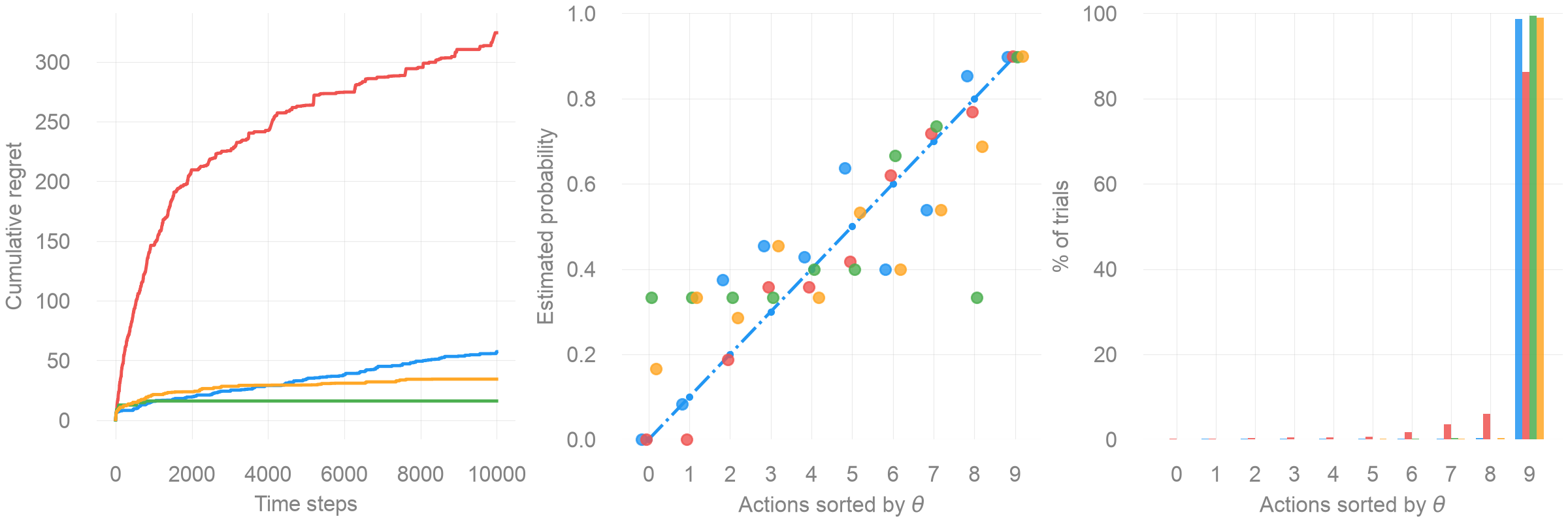

Figure 1: The results of the experiment on solving Bernoulli bandit with K=10, slot machines with reward probabilities, {0.0, 0.1, …, 0.9}. Each solver runs 10,000 steps.

The three panels in Figure 1 show cumulative pseudo-regret, final reward-probability estimates, and the fraction of pulls assigned to each arm.

Cumulative Regret

Lower curves indicate less expected reward lost relative to always selecting the arm with probability \(0.9\). In this realization, the final ordering from lowest to highest regret is Thompson Sampling, the Bayesian UCB-style heuristic, \(\epsilon\)-greedy, and the UCB1-style implementation. That ordering describes this run only.

Probability Estimates

The middle panel compares each final estimate with the true arm probabilities. Estimates for rarely selected arms remain noisy because reward maximization does not require every probability to be estimated equally well. In particular, a UCB arm is not permanently abandoned when its bonus shrinks: if its count stays fixed, the \(\ln t\) term can increase its score and cause another visit.

Pull Fractions

The right panel makes the exploration policies visible. With \(\epsilon=0.01\), \(\epsilon\)-greedy continues to assign random pulls to all arms. The two UCB-style policies allocate pulls according to their optimism bonuses, while Thompson Sampling allocates them through posterior samples. All four concentrate most trials on the best arm in this run, but to different degrees.

Limits of the Comparison

The benchmark uses one seed, one set of arm probabilities, and one parameter setting per method. Its curves illustrate behavior but cannot establish a general ranking or show that one uncertainty model is more efficient. A stronger comparison would repeat every solver across many seeds and bandit instances, then report mean regret with uncertainty intervals.

Conclusion

The main distinction among these methods is how they decide that an arm deserves another pull. \(\epsilon\)-greedy explores at random, UCB adds an optimism bonus, and Thompson Sampling acts on posterior samples. The plotted run shows how those choices affect regret and sampling frequency, but it is evidence about one controlled example rather than a universal performance ranking.

For a comparative experiment, the next step would be to repeat the simulation across seeds and problem instances. For understanding the algorithms, this single run already exposes the useful mechanism: exploration can be scheduled randomly, driven by a confidence bonus, or induced by posterior uncertainty.

Appendix

Method	Exploration mechanism	Reward model
\(\epsilon\)-greedy	Random action with probability \(\epsilon\)	Empirical arm means
UCB1-style implementation	Count-based optimism bonus	Empirical arm means
Bayesian UCB-style heuristic	Beta posterior mean plus scale bonus	Beta-Bernoulli
Thompson Sampling	Posterior sampling	Beta-Bernoulli

References

Auer, Peter, Nicolò Cesa-Bianchi, and Paul Fischer. 2002. “Finite-Time Analysis of the Multiarmed Bandit Problem.” Machine Learning 47: 235–56. https://doi.org/10.1023/A:1013689704352.

Kaufmann, Emilie, Olivier Cappé, and Aurélien Garivier. 2012. “On Bayesian Upper Confidence Bounds for Bandit Problems.” Proceedings of the Fifteenth International Conference on Artificial Intelligence and Statistics, Proceedings of machine learning research, vol. 22: 592–600. https://proceedings.mlr.press/v22/kaufmann12.html.

Thompson, William R. 1933. “On the Likelihood That One Unknown Probability Exceeds Another in View of the Evidence of Two Samples.” Biometrika 25 (3-4): 285–94. https://doi.org/10.1093/biomet/25.3-4.285.