Reinforcement Learning: Tabular Q-Learning

code

python

mdp

reinforcement learning

Author

Gregor Cerar

Published

2025-12-17

Abstract

This post implements tabular Q-learning for deterministic FrozenLake environments in Gymnasium. It connects the update equation to the training loop and explains what the stored state, action, Q-value, reward, and episode-length plots measure.

I used the official Gymnasium tabular Q-learning tutorial as a starting point for learning reinforcement learning. Q-learning is small enough to implement with a NumPy table, while FrozenLake exposes the essential pieces: states, actions, transitions, sparse rewards, exploration, and terminal states.

This post connects those pieces to the update equation, walks through the implementation, and explains how to read the stored experiment figures.

The Frozen Lake Environment

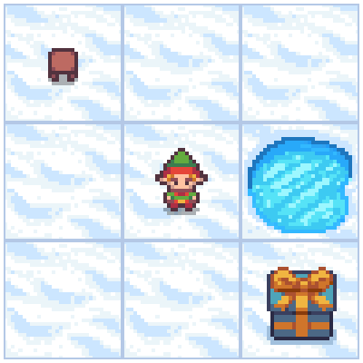
FrozenLake is a small grid environment in which an elf must move from the starting tile in the top-left corner to a present in the bottom-right corner without entering a hole.

The environment can also be slippery. In that mode, the selected direction and its two perpendicular directions each occur with probability one third. The experiments below instead set is_slippery=False, so transitions are deterministic.

Action Space

Gymnasium represents the action space as Discrete(4) with the following integer mapping:

0: left,
1: down,
2: right,
3: up.

The value passed to env.step is therefore one scalar integer, not a vector.

Observation Space

The observation returned by the environment represents the agent’s current position on the grid. Since Frozen Lake consists of a finite number of discrete tiles, each tile is assigned a unique integer identifier.

For example, a $3\times{}3$ grid is indexed as:

\[ \begin{matrix} 0 & 1 & 2 \\ 3 & 4 & 5 \\ 6 & 7 & 8 \end{matrix} \]

More generally, the tile index can be computed as:

\[ \text{tile}(r,c) = r \cdot N_{\text{cols}} + c, \]

where:

$r$ is the row index,
$c$ is the column index,
$N_{\text{cols}}$ is the number of columns in the grid.

This discrete state representation makes Frozen Lake particularly well-suited for tabular methods such as Q-learning.

Rewards

The default reward structure is sparse:

$+1$ for reaching the goal tile,
$0$ for stepping onto a frozen tile,
$0$ for falling into a hole.

The agent therefore receives no positive feedback until it reaches the goal. Exploration matters because an unvisited state-action pair remains indistinguishable from every other zero-valued entry in the initial Q-table.

For full details, see the official Frozen Lake environment documentation.

Reinforcement Learning Formulation

Frozen Lake can be formalized as a finite Markov Decision Process (MDP) defined by the tuple $(\mathcal{S}, \mathcal{A}, \mathcal{P}, \mathcal{R}, \gamma)$.

State Space $\mathcal{S}$

The state space consists of all discrete tiles on the grid:

\[ \mathcal{S} = \{ 0, 1, \dots, (N_\text{rows}\cdot N_\text{cols}-1) \}. \]

Each state uniquely represents the agent’s current position in the lake.

Action Space $\mathcal{A}$

At each time step, the agent can choose one of four actions:

\[ \mathcal{A} = \{ \text{left}, \text{down}, \text{right}, \text{up} \}. \]

These actions correspond to deterministic intentions, even though the actual transition may be stochastic when the lake is slippery.

Transition Dynamics $P(s'|s,a)$

The transition function defines the probability of moving from state $s$ to state $s'$ after taking action $a$.

In the non-slippery version used below, the intended transition is deterministic.
In the slippery version, the intended direction and the two perpendicular directions each have probability one third.

The deterministic setting isolates the Q-learning mechanics. Enabling slippery transitions would test the same algorithm under transition uncertainty.

Reward Function $R(s, a, s')$

The reward function is sparse and simple:

\[ R(s, a, s') = \begin{cases} 1, & \text{if $s'$ is the goal state},\\ 0, & \text{otherwise}. \end{cases} \]

Episodes terminate when the agent reaches the goal or falls into a hole.

from dataclasses import dataclass
from pathlib import Path

import gymnasium as gym
import matplotlib.pyplot as plt
import numpy as np
import pandas as pd
import seaborn as sns
from aquarel import load_theme
from gymnasium.envs.toy_text.frozen_lake import generate_random_map
from matplotlib.figure import Figure
from tqdm.auto import tqdm, trange

DPI = 200  # 2x the ~800px content column, so figures stay crisp on HiDPI screens
FIGURES = Path("./figures")


def save_fig(fig: Figure, name: str) -> None:
    """Write a figure into figures/ as lossless WebP, keeping the transparent background."""
    FIGURES.mkdir(parents=True, exist_ok=True)
    fig.savefig(FIGURES / name, dpi=DPI, transparent=True, pil_kwargs={"lossless": True, "method": 6})
    plt.close(fig)

@dataclass(frozen=True, slots=True)
class Params:
    n_runs: int = 20  # number of runs from scratch
    total_episodes: int = 2_000  # total episodes (# of playthroughs) in the same run
    learning_rate: float = 0.8  # Q-Learning learning rate
    gamma: float = 0.95  # discounting rate
    epsilon: float = 0.1  # probability of exploration vs. exploitation
    proba_frozen: float = 0.9  # probability that a tile is frozen (not a hole)
    is_slippery: bool = False  # enables slipping: 1/3 forward, 1/3 left, 1/3 right
    seed: int = 123  # seed for reproducibility

SHOW_PROGRESS: bool = False

Q-learning Update

Q-learning stores an estimate $Q(s,a)$ of the discounted return obtained by choosing action $a$ in state $s$ and then following the best available actions. The tabular update is (Watkins and Dayan 1992):

\[ Q(s_t,a_t) \leftarrow Q(s_t,a_t) + \alpha \left[r_{t+1} + \gamma(1-d_t)\max_{a'}Q(s_{t+1},a') - Q(s_t,a_t)\right], \]

where $\alpha$ is the learning rate, $\gamma$ is the discount factor, and $d_t$ is one when the transition terminates the episode. The bracketed term is the temporal-difference error: the observed reward plus the best estimated next-state value, minus the current estimate.

The Qlearning.update method implements this equation directly. It sets the next-state value to zero for a terminal goal or hole, preventing value from leaking beyond the end of an episode. A time-limit truncation is handled separately and still bootstraps from the observed next state.

Exploration Policy

The EpsilonGreedy class explores with probability $\epsilon=0.1$ and otherwise chooses an action with the largest current Q-value. When several actions tie, it samples uniformly among them; this matters initially because every table entry starts at zero.

Implementation

class Qlearning:
    qtable: np.ndarray

    def __init__(self, lr: float, gamma: float, state_size: int, action_size: int) -> None:
        self.lr = lr
        self.gamma = gamma
        self.state_size = state_size
        self.action_size = action_size
        self.reset_qtable()

    def update(self, state: int, action: int, reward: float, new_state: int, terminated: bool) -> float:
        """Update Q(s,a) := Q(s,a) + lr * [R(s,a) + gamma * max Q(s',a') - Q(s,a)]"""
        next_value = 0.0 if terminated else np.max(self.qtable[new_state, :])
        delta = reward + self.gamma * next_value - self.qtable[state, action]

        q_update = self.qtable[state, action] + self.lr * delta
        return q_update

    def reset_qtable(self) -> None:
        """Reset the Q-table."""
        self.qtable = np.zeros((self.state_size, self.action_size))


class EpsilonGreedy:
    def __init__(self, epsilon: float, seed: int | None) -> None:
        self.eps = epsilon
        self.rng = np.random.default_rng(seed)

    def choose_action(self, action_space: gym.spaces.Space, state: int, qtable: np.ndarray) -> int:
        """Choose an action `a` in the current world state (s)."""
        action: int

        # random number decides whether we do ...
        explore_exploit_tradeoff = self.rng.uniform(0, 1)
        if explore_exploit_tradeoff < self.eps:  # ... exploration (random action) ...
            action = action_space.sample()
        else:  # ... or exploitation (use direction with the biggest Q-value for this state)
            (max_ids,) = np.where(qtable[state, :] == max(qtable[state, :]))
            action = self.rng.choice(max_ids)  # pick one if multiple directions with max probability

        return action

Training Loop

Each run starts from a zero-filled Q-table. For every episode, the loop resets the environment, alternates between epsilon-greedy action selection and the Q-learning update, and stops at a goal, hole, or time limit.

The experiment records total reward and episode length for every episode. It also records every visited state and selected action across training, then saves the final Q-table from each run. Those distinctions matter later: visit distributions describe the full learning process, whereas the averaged Q-table summarizes the final tables.

The default configuration uses 20 runs of 2,000 episodes each, a learning rate of 0.8, discount factor of 0.95, fixed exploration probability of 0.1, and deterministic transitions.

def run_env(env: gym.Env, learner: Qlearning, explorer: EpsilonGreedy, p: Params, state_size: int, action_size: int):
    rewards = np.zeros((p.total_episodes, p.n_runs), dtype=float)
    steps = np.zeros((p.total_episodes, p.n_runs), dtype=int)
    episodes = np.arange(p.total_episodes, dtype=int)

    qtables = np.zeros((p.n_runs, state_size, action_size), dtype=float)

    all_states: list[int] = []
    all_actions: list[int] = []

    for run in trange(p.n_runs, leave=False, disable=(not SHOW_PROGRESS)):
        learner.reset_qtable()

        for episode in tqdm(episodes, leave=False, disable=(not SHOW_PROGRESS)):
            state, _ = env.reset(seed=p.seed)
            step: int = 0
            done: bool = False
            total_rewards: float = 0.0

            while not done:
                action = explorer.choose_action(action_space=env.action_space, state=state, qtable=learner.qtable)

                # log all the stats and actions
                all_states.append(state)
                all_actions.append(action)

                # take the action $a$ and observe the outcome state $s'$ and reward $r$
                new_state, reward, terminated, truncated, info = env.step(action)

                # Mark the episode as done if the game terminated (victory/hole) or was truncated (wall)
                done = terminated or truncated

                # learner updates Q-table; only bootstrap from the next state if the episode
                # didn't actually end there (truncation still bootstraps, termination doesn't)
                learner.qtable[state, action] = learner.update(state, action, float(reward), new_state, terminated)

                total_rewards += float(reward)
                step += 1

                # our new state is state
                state = new_state

            # log all rewards and steps
            rewards[episode, run] = total_rewards
            steps[episode, run] = step

        qtables[run, :, :] = learner.qtable

    return rewards, steps, episodes, qtables, all_states, all_actions

def postprocess(episodes: np.ndarray, params: Params, rewards: np.ndarray, steps: np.ndarray, map_size: int):
    """Convert the results of the simulation into dataframes."""

    res = pd.DataFrame(
        data={
            "Episodes": np.tile(episodes, reps=params.n_runs),
            "Rewards": rewards.flatten(order="F"),
            "Steps": steps.flatten(order="F"),
        }
    )
    res["cum_rewards"] = rewards.cumsum(axis=0).flatten(order="F")
    res["map_size"] = np.repeat(f"{map_size}x{map_size}", res.shape[0])

    st = pd.DataFrame(data={"Episodes": episodes, "Steps": steps.mean(axis=1)})
    st["map_size"] = np.repeat(f"{map_size}x{map_size}", st.shape[0])

    return res, st

def qtable_directions_map(qtable: np.ndarray, map_size: int):
    """Get the best learned action & map it to arrows."""

    eps = np.finfo(qtable.dtype).eps  # minimum float number on the machine
    directions = {0: "←", 1: "↓", 2: "→", 3: "↑"}

    qtable_val_max = qtable.max(axis=1).reshape(map_size, map_size)
    qtable_best_action = np.argmax(qtable, axis=1).reshape(map_size, map_size)
    qtable_directions = np.empty(qtable_best_action.size, dtype=str)

    for idx, val in enumerate(qtable_best_action.flat):
        if qtable_val_max.flat[idx] > eps:
            # Assign an arrow only if a minimal Q-value has been learned as best action
            # otherwise since 0 is a direction, it also gets mapped on the tiles where
            # it didn't actually learn anything
            qtable_directions[idx] = directions[val]

    qtable_directions = qtable_directions.reshape(map_size, map_size)
    return qtable_val_max, qtable_directions

def plot_q_values_map(qtable: np.ndarray, env: gym.Env, map_size: int):
    """Plot the last frame of the simulation and the policy learned."""

    qtable_val_max, qtable_directions = qtable_directions_map(qtable, map_size)

    fig, ax = plt.subplots(nrows=1, ncols=2, figsize=(10, 5.5), constrained_layout=True)

    ax[0].imshow(env.render(), aspect="equal", interpolation="none")
    ax[0].axis("off")
    ax[0].set_title("Last frame")

    # Plot the policy
    sns.heatmap(
        qtable_val_max,
        annot=qtable_directions,
        fmt="",
        square=True,
        ax=ax[1],
        cmap=sns.color_palette("Blues", as_cmap=True),
        linewidths=0.5,
        linecolor="black",
        xticklabels=[],
        yticklabels=[],
    )
    ax[1].set(title="Learned Q-values\nArrows represent best action")
    ax[1].axis("off")

    # autoscale annotation font size
    rows, cols = qtable_val_max.shape
    bbox = ax[0].get_window_extent().transformed(fig.dpi_scale_trans.inverted())
    width_in, height_in = bbox.width, bbox.height

    # Heuristic scaling factor (tweak as needed)
    scale = min(width_in / cols, height_in / rows)
    fontsize = scale * 50

    # Apply new font size
    for text in ax[1].texts:
        text.set_fontsize(fontsize)

    for _, spine in ax[1].spines.items():
        spine.set_visible(True)
        spine.set_linewidth(0.7)
        spine.set_color("black")

    return fig, ax

def plot_states_actions_distribution(states: list[int], actions: list[int], map_size: int):
    """Plot the distributions of states and actions."""
    labels = {"LEFT": 0, "DOWN": 1, "RIGHT": 2, "UP": 3}

    fig, ax = plt.subplots(nrows=1, ncols=2, figsize=(11, 5), constrained_layout=True)
    sns.histplot(data=states, ax=ax[0], kde=True)
    ax[0].set_title("States")

    sns.histplot(data=actions, ax=ax[1])
    ax[1].set_xticks(list(labels.values()), labels=labels.keys())
    ax[1].set_title("Actions")

    return fig, ax

def plot_steps_and_rewards(rewards_df: pd.DataFrame, steps_df: pd.DataFrame):
    """Plot the steps and rewards from dataframes."""
    fig, ax = plt.subplots(nrows=1, ncols=2, figsize=(11, 5), constrained_layout=True)
    sns.lineplot(data=rewards_df, x="Episodes", y="cum_rewards", hue="map_size", linewidth=0.7, ax=ax[0])
    ax[0].set(ylabel="Cumulated rewards")

    sns.lineplot(data=steps_df, x="Episodes", y="Steps", hue="map_size", linewidth=0.7, ax=ax[1])
    ax[1].set(ylabel="Averaged steps number")

    for axi in ax:
        axi.legend(title="map size")

    return fig, ax

from collections.abc import Callable

EnvFactory = Callable[[int], gym.Env]


def run_experiments(make_env: EnvFactory, params: Params, map_sizes: list[int] | int, prefix: str):
    res_all = pd.DataFrame()
    st_all = pd.DataFrame()

    if isinstance(map_sizes, int):
        map_sizes = [map_sizes]

    for map_size in map_sizes:
        env = make_env(map_size)

        action_size: int | None = getattr(env.action_space, "n", None)
        assert action_size is not None

        state_size: int | None = getattr(env.observation_space, "n", None)
        assert state_size is not None

        env.action_space.seed(params.seed)  # Set the seed to get reproducible results when sampling the action space
        learner = Qlearning(
            lr=params.learning_rate, gamma=params.gamma, state_size=state_size, action_size=action_size
        )
        explorer = EpsilonGreedy(epsilon=params.epsilon, seed=params.seed)

        print(f"Map size: {map_size}x{map_size}")
        rewards, steps, episodes, qtables, all_states, all_actions = run_env(
            env, learner, explorer, params, state_size, action_size
        )

        # Save the results in dataframes
        res, st = postprocess(episodes, params, rewards, steps, map_size)
        res_all = pd.concat([res_all, res])
        st_all = pd.concat([st_all, st])
        qtable = qtables.mean(axis=0)  # Average the Q-table between runs

        with load_theme("ambivalent"):
            fig, _ = plot_states_actions_distribution(states=all_states, actions=all_actions, map_size=map_size)
        save_fig(fig, f"{prefix}-states-actions-{map_size}.webp")

        with load_theme("ambivalent"):
            fig, _ = plot_q_values_map(qtable, env, map_size)
        save_fig(fig, f"{prefix}-q-values-{map_size}.webp")

        env.close()

    with load_theme("ambivalent"):
        fig, _ = plot_steps_and_rewards(res_all, st_all)
    save_fig(fig, f"{prefix}-steps-rewards.webp")

def make_frozenlake_env(params: Params) -> EnvFactory:
    def _factory(map_size: int) -> gym.Env:
        return gym.make(
            "FrozenLake-v1",
            is_slippery=params.is_slippery,
            render_mode="rgb_array",
            desc=generate_random_map(size=map_size, p=params.proba_frozen, seed=params.seed),
            # reward_schedule=(10.0, -1.0, -0.01),  # reach goal, reach hole, reach frozen (includes Start)
        )

    return _factory


map_sizes = [4, 7, 9, 11]
params = Params()

run_experiments(make_frozenlake_env(params), params, map_sizes, prefix="main")

Map size: 4x4
Map size: 7x7
Map size: 9x9
Map size: 11x11

Results

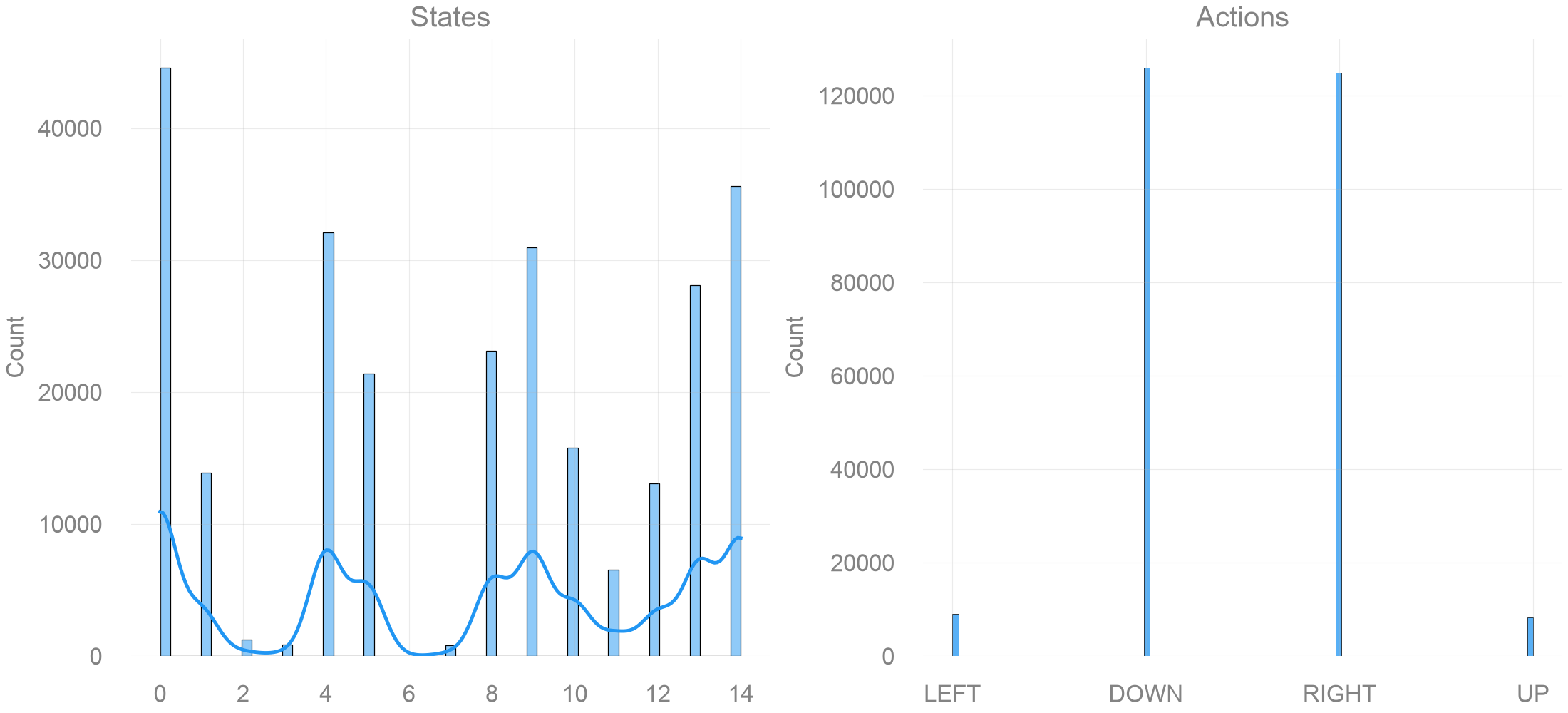
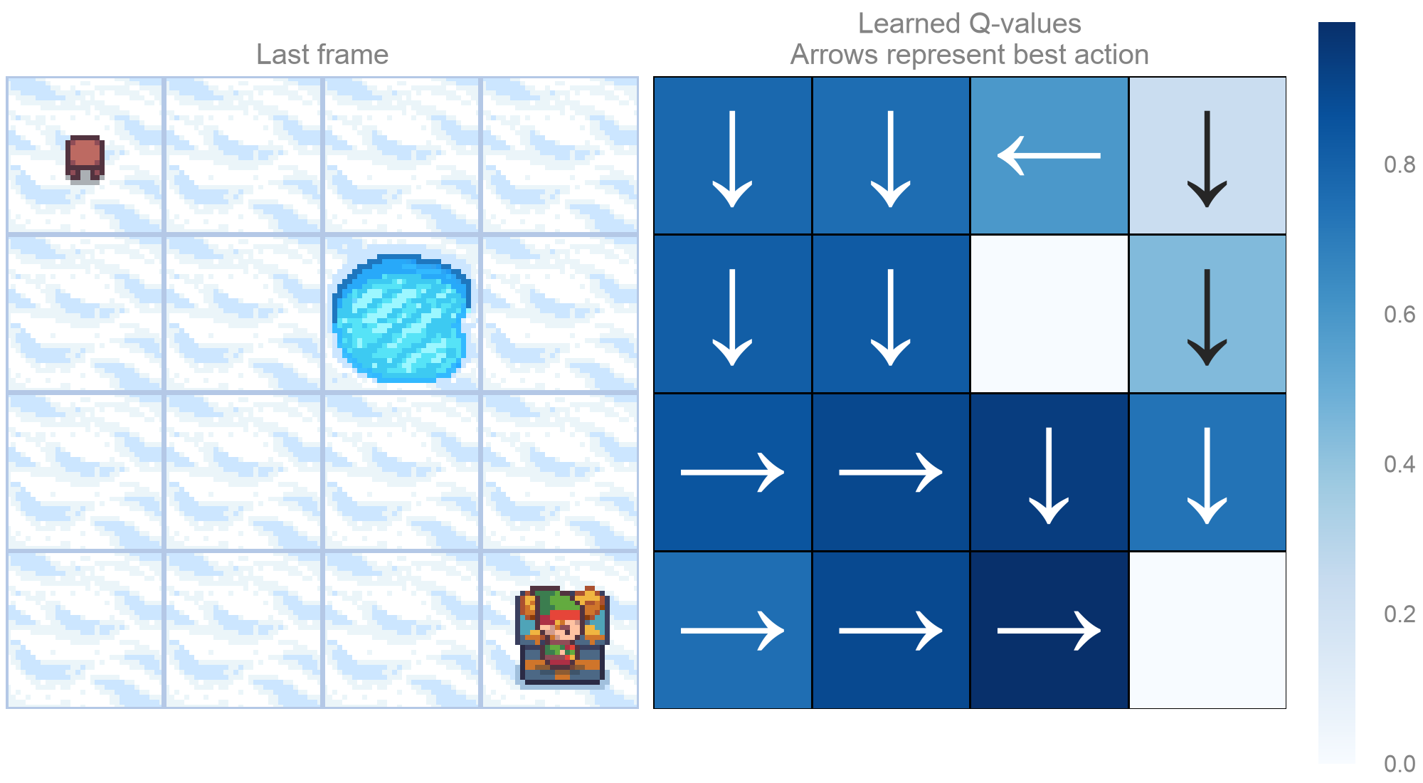
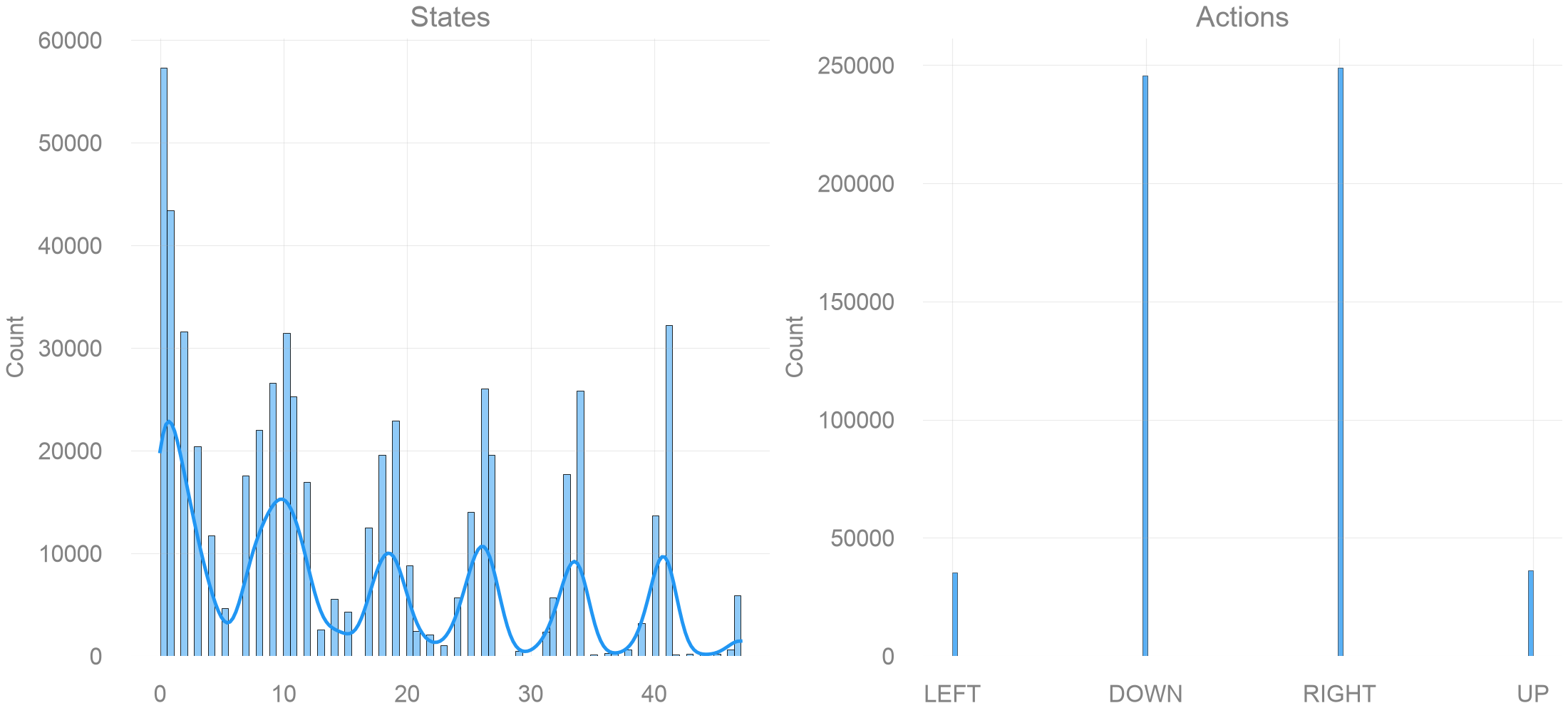
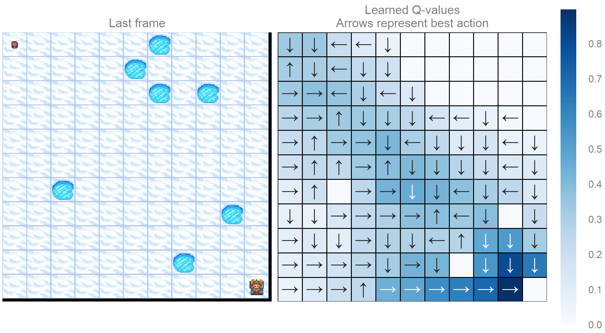
The main experiment evaluates fixed 4x4, 7x7, 9x9, and 11x11 maps generated with the same seed and a 0.9 probability that each sampled tile is safe. Each pair of figures combines data from all 20 runs.

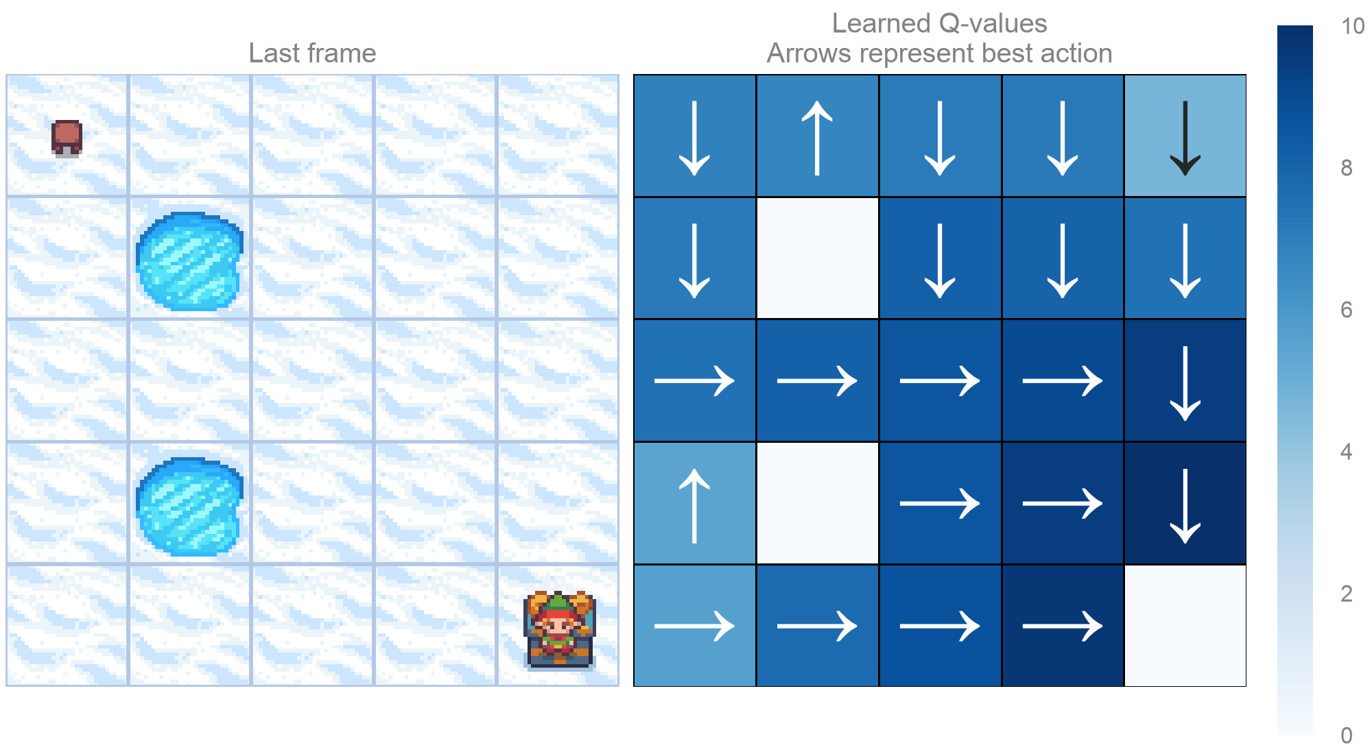
The state and action distributions aggregate all visits during training, so they mix early exploration with later exploitation. The Q-value panels display the mean final Q-table across runs. Averaging makes broad patterns easier to see but can blur policies that selected different actions in the same state.

The figures provide a qualitative record of these runs; the notebook does not store summary tables or confidence intervals, so I do not use them to claim a precise performance difference between map sizes.

Last frame and learned Q-values, 4x4 map

Last frame and learned Q-values, 7x7 map

Last frame and learned Q-values, 9x9 map

State and action distributions, 11x11 map

Last frame and learned Q-values, 11x11 map

Cumulative rewards and mean episode lengths across map sizes.

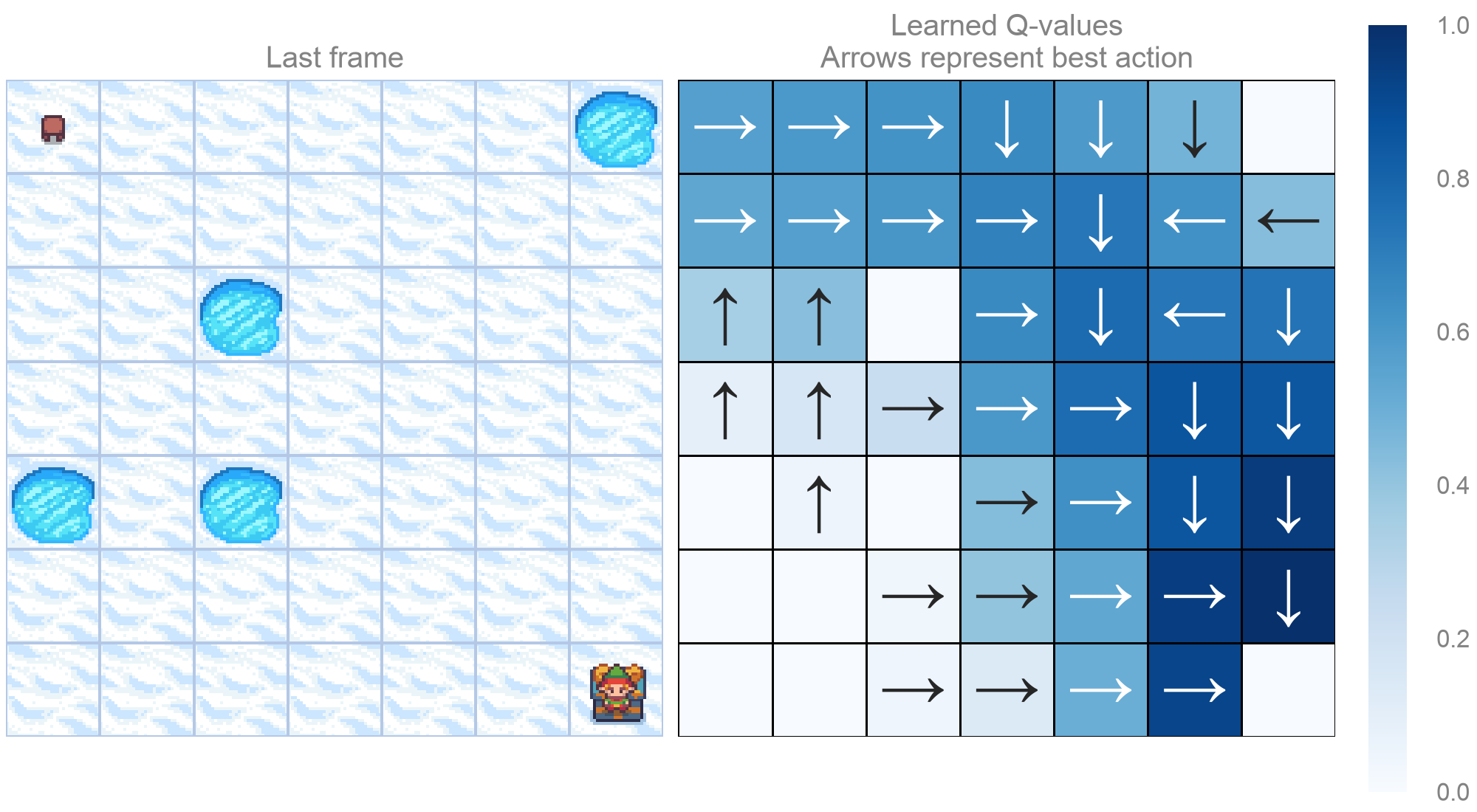
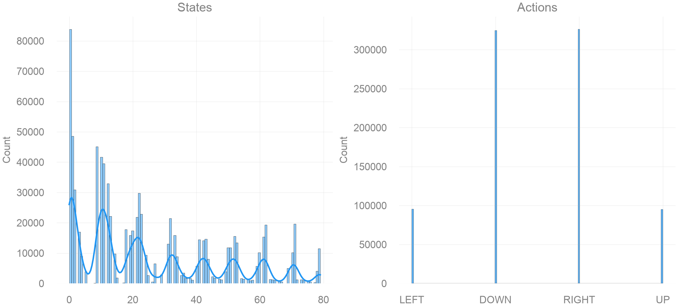
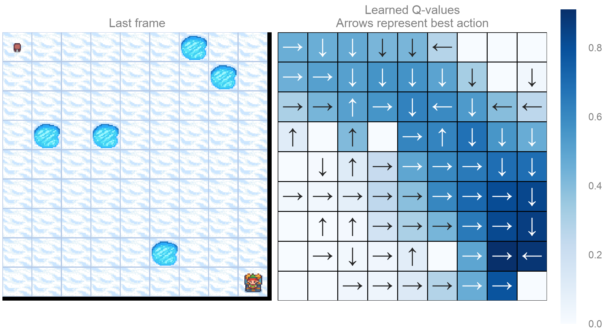
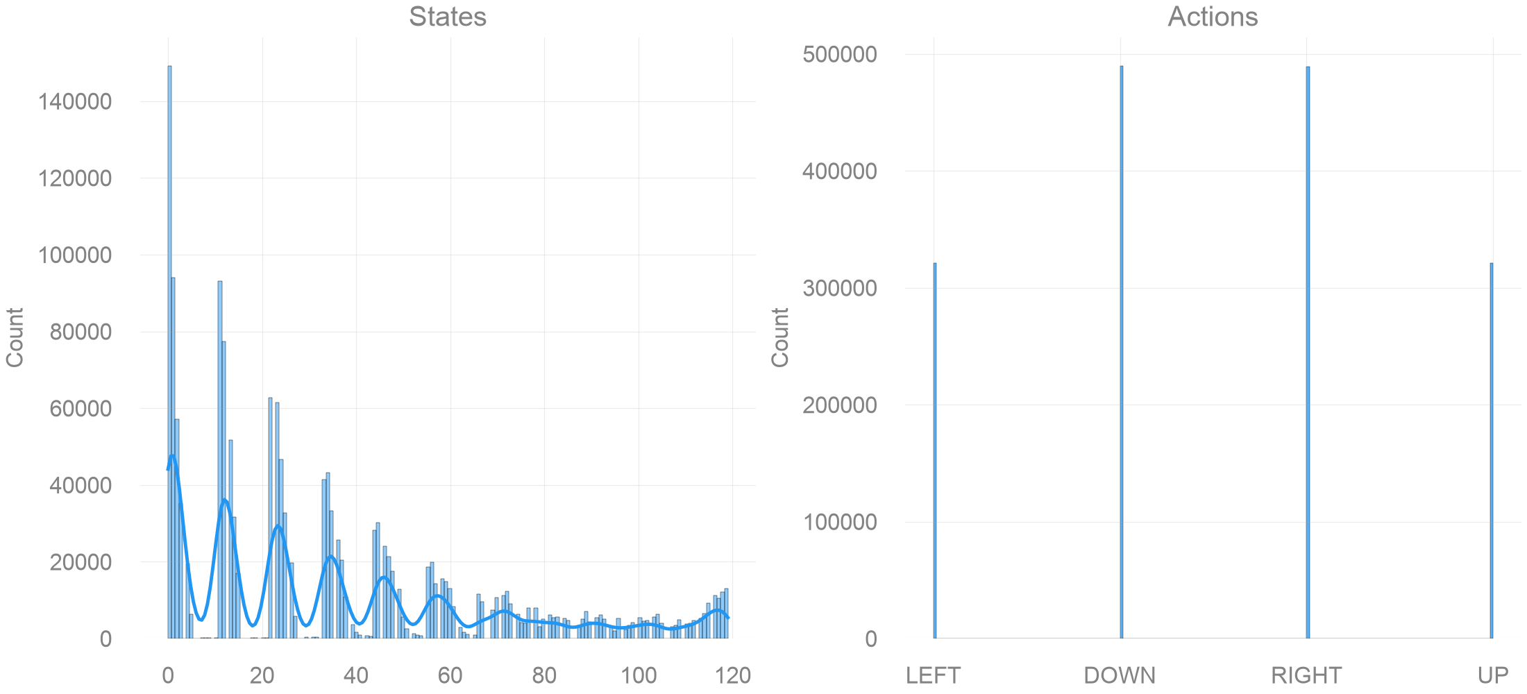
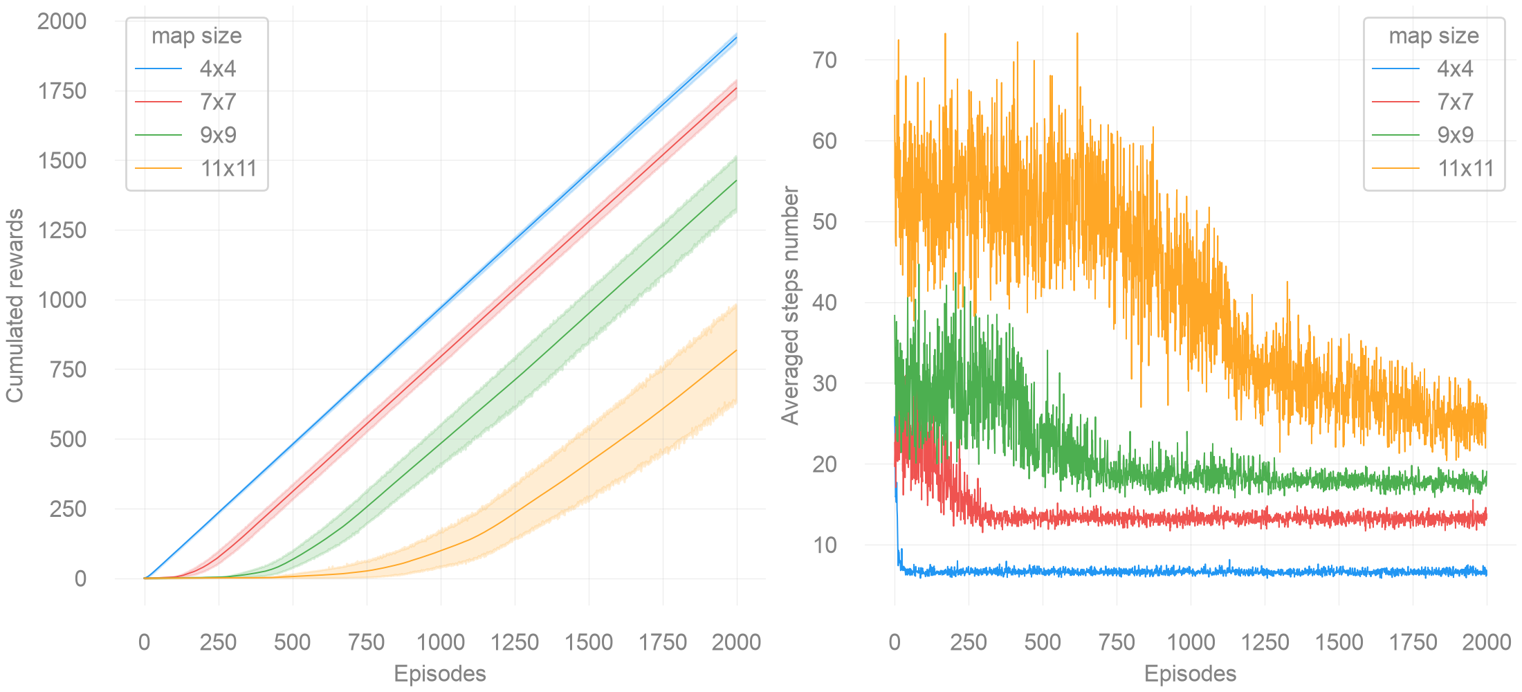
With the default reward schedule, cumulative reward is also cumulative success count because only a goal contributes one point. Its slope indicates how frequently recent episodes reached the goal. Mean episode length needs more care: a short episode may represent either an efficient route to the goal or an early fall into a hole.

Conclusions

This implementation connects each part of tabular Q-learning to a visible quantity: the Q-table stores action values, epsilon-greedy sampling generates experience, and the temporal-difference update moves one table entry toward a reward-plus-next-value target. FrozenLake keeps those mechanics inspectable because every state-action value fits in a small matrix.

The experiment is deliberately limited. It uses deterministic transitions, fixed hyperparameters, one generated map per size, and no held-out evaluation phase. The stored plots describe these training runs rather than establishing how Q-learning scales across FrozenLake problems.

Reward-Shaping Experiment

The additional experiment changes the reward schedule to $+10$ for the goal, $-10$ for a hole, and $-0.01$ for every other transition. This supplies feedback before the first success, but it also changes the objective by explicitly penalizing holes and longer routes.

It uses 5x5 and 25x25 maps rather than the sizes in the main experiment, so the figures are an exploratory extension rather than a controlled comparison with the sparse-reward runs.

Stored Results

SHOW_PROGRESS = False


def make_frozenlake_env(params: Params) -> EnvFactory:
    def _factory(map_size: int) -> gym.Env:
        return gym.make(
            "FrozenLake-v1",
            is_slippery=params.is_slippery,
            render_mode="rgb_array",
            desc=generate_random_map(size=map_size, p=params.proba_frozen, seed=params.seed),
            reward_schedule=(10.0, -10.0, -0.01),  # reach goal, reach hole, reach frozen (includes Start)
        )

    return _factory


params = Params()

run_experiments(make_frozenlake_env(params), params, map_sizes=[5, 25], prefix="shaped")

Map size: 5x5
Map size: 25x25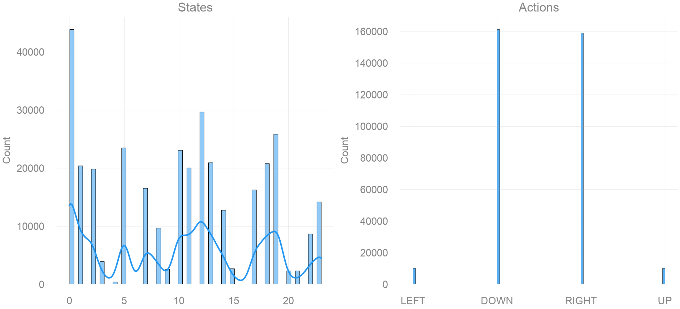

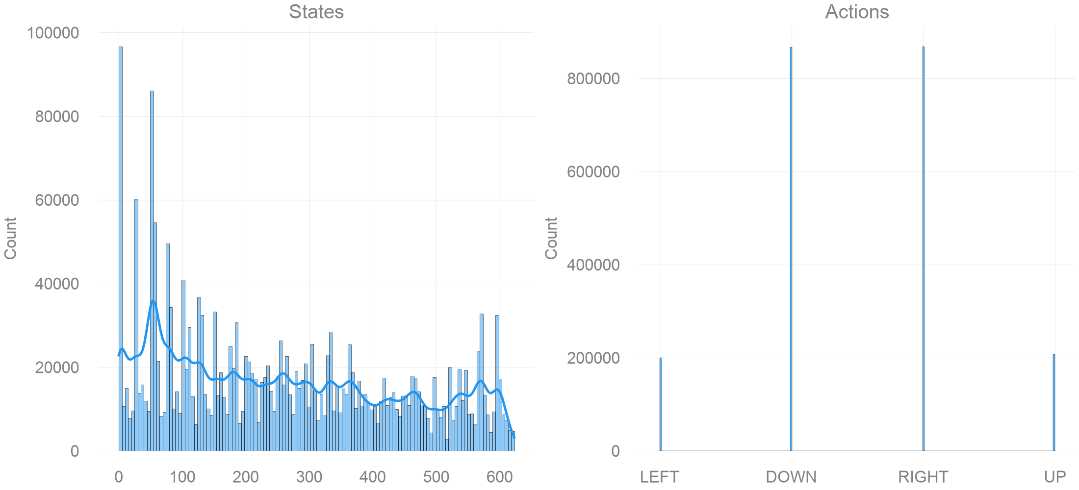
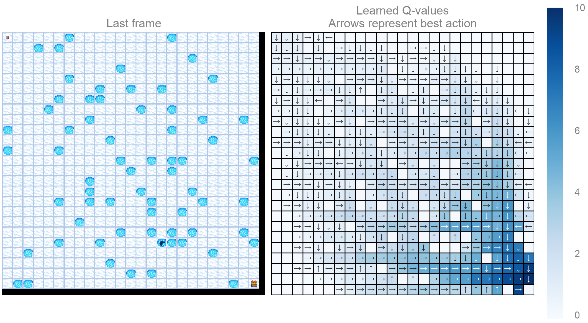
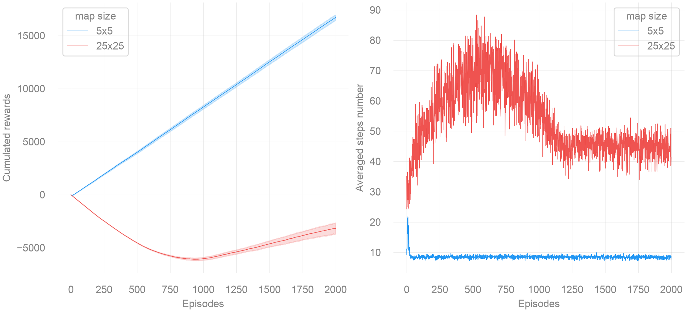
Last frame and learned Q-values, 5x5 map

State and action distributions, 25x25 map

Last frame and learned Q-values, 25x25 map

Cumulative shaped rewards and mean episode lengths for the 5x5 and 25x25 maps.

Cumulative shaped reward is not a success count: it combines goal bonuses, hole penalties, and per-step costs. It therefore cannot be compared numerically with cumulative reward in the main experiment without separating those components.

References

Watkins, Christopher J. C. H., and Peter Dayan. 1992. “Q-Learning.” Machine Learning 8: 279–92. https://doi.org/10.1007/BF00992698.

Reuse

CC BY-NC-SA 4.0