Diffusion Models

Abstract

A worked implementation of a small DDPM and classifier-free guidance, with attention to the assumptions, shortcuts, and limits that affect the results.

Introduction

I worked through the first four modules of NVIDIA’s Generative AI with Diffusion Models: U-Net architecture, the DDPM forward and reverse processes, architectural refinements, and classifier-free guidance.

This post uses my cleaned-up workshop implementation to examine what each part actually does. The main lesson is that the code is useful as a compact teaching model, but several results need narrow interpretation: the architecture changes are not an ablation study, the short noise schedule does not fully erase the input, and the guidance experiment contains one sample per setting.

The dataset is FashionMNIST resized to 16x16. That keeps training short enough for an exploratory run while leaving enough structure to judge whether the generated samples resemble garments.

Experimental Setup

The notebook concatenates FashionMNIST’s 60,000 training images and 10,000 test images because it does not report held-out metrics. It resizes every image to 16x16, applies random horizontal flips, scales pixels to \([-1,1]\), and trains with batches of 128.

The diffusion schedule has \(T=150\) steps and increases \(\beta_t\) linearly from \(0.0001\) to \(0.02\). This corrupts the images heavily, but the last panel in the forward-process figure still retains visible structure. The endpoint is therefore not equivalent to pure Gaussian noise. Sampling nevertheless starts from \(\mathcal{N}(0,\mathbf{I})\), and that mismatch may contribute to the rough samples in this small experiment.

nrows = 10
ncols = 15

T = nrows * ncols
B_start = 0.0001
B_end = 0.02
B = torch.linspace(B_start, B_end, T).to(device)

def load_dataset(img_size: int, batch_size: int) -> tuple[ConcatDataset, DataLoader]:
    from torchvision.datasets import FashionMNIST

    transform = VT.Compose(
        [
            VT.Resize((img_size, img_size)),
            VT.ToTensor(),  # Scales data into [0,1]
            VT.RandomHorizontalFlip(),
            VT.Lambda(lambda t: (t * 2) - 1),  # Scale between [-1, 1]
        ]
    )

    train_set = FashionMNIST(DATASET_PATH, train=True, download=True, transform=transform)
    test_set = FashionMNIST(DATASET_PATH, train=False, download=True, transform=transform)
    dataset = ConcatDataset([train_set, test_set])
    dataloader = DataLoader(dataset, batch_size=batch_size, drop_last=True, **loader_kwargs)
    return dataset, dataloader


dataset, dataloader = load_dataset(IMG_SIZE, BATCH_SIZE)

Architecture

The denoiser is a small U-Net, an encoder-decoder with skip connections originally introduced for biomedical image segmentation (Ronneberger et al. 2015). It receives a noisy image and a timestep and predicts the noise component in that image.

The workshop changes five parts of its baseline architecture at once. The resulting samples look different, but this comparison is not an ablation study, so it cannot identify which change caused a particular improvement.

1. GELU replaces ReLU. ReLU returns zero for negative inputs, whereas GELU changes smoothly around zero and retains small negative outputs (Hendrycks and Gimpel 2016). This changes the optimization behavior, but this notebook does not isolate its effect on sample quality.
2. GroupNorm replaces BatchNorm. GroupNorm calculates statistics within each sample rather than across a batch (Wu and He 2018). Its output therefore does not depend on which noise levels happen to share a batch.
3. Space-to-depth replaces MaxPool. A rearrangement moves each 2x2 neighborhood into the channel dimension before a learned convolution combines those values. The rearrangement itself is lossless; the following channel-reducing convolution is not.
4. Sinusoidal features encode the timestep. Fixed sine and cosine features expose several scales before a learned embedding network (Vaswani et al. 2017). They provide a structured time representation, but they do not by themselves guarantee that every timestep is easy to distinguish.
5. A residual path skips one convolution. In ResidualConvBlock, the output of the first convolution is added to the output of the second. This is a shorter path than passing through both convolutions, although it is not a skip from the raw block input.

Checkerboard artifacts have a more specific cause than this list suggests. Uneven overlap in some transposed convolutions can give output pixels different numbers of contributing inputs (Odena et al. 2016). This U-Net still uses transposed convolutions, but its kernel_size=2, stride=2 configuration tiles without overlap. The space-to-depth block addresses downsampling and information flow, not that upsampling artifact directly.

class GELUConvBlock(nn.Module):
    def __init__(self, in_chs: int, out_chs: int, group_size: int) -> None:
        super().__init__()
        self.layers = nn.Sequential(
            nn.Conv2d(in_chs, out_chs, kernel_size=3, stride=1, padding=1),
            nn.GroupNorm(group_size, out_chs),
            nn.GELU(),
        )

    def forward(self, x: Tensor) -> Tensor:
        return self.layers(x)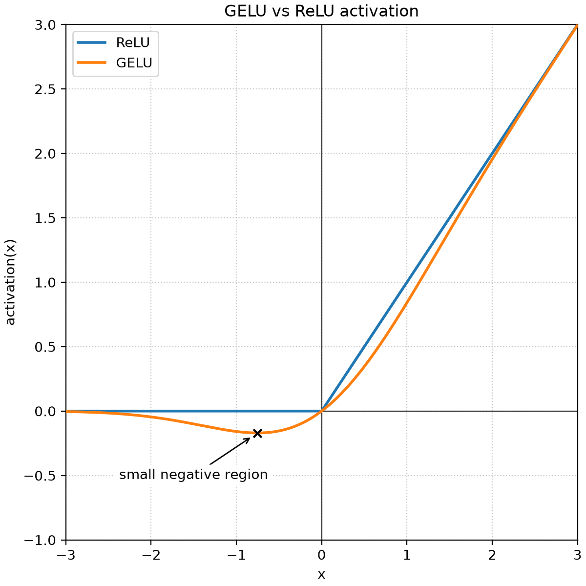

Figure 1: GELU and ReLU over the interval \([-3,3]\).

Learned Downsampling

RearrangePoolBlock first converts a tensor of shape \((B,C,H,W)\) into \((B,4C,H/2,W/2)\). This space-to-depth step only reorders values. A GELUConvBlock then maps \(4C\) channels back to \(C\), allowing a learned compression instead of MaxPool’s fixed maximum operation.

The complete block is neither lossless nor the inverse of the upsampling path because its convolution reduces the channel count. Its practical role is to preserve all four spatial values until the network learns how to combine them.

import einops

x = torch.rand(128, 3, 128, 128)
y = einops.rearrange(x, "b c (h p1) (w p2) -> b (c p1 p2) h w", p1=2, p2=2)

assert np.prod(x.shape) == np.prod(y.shape)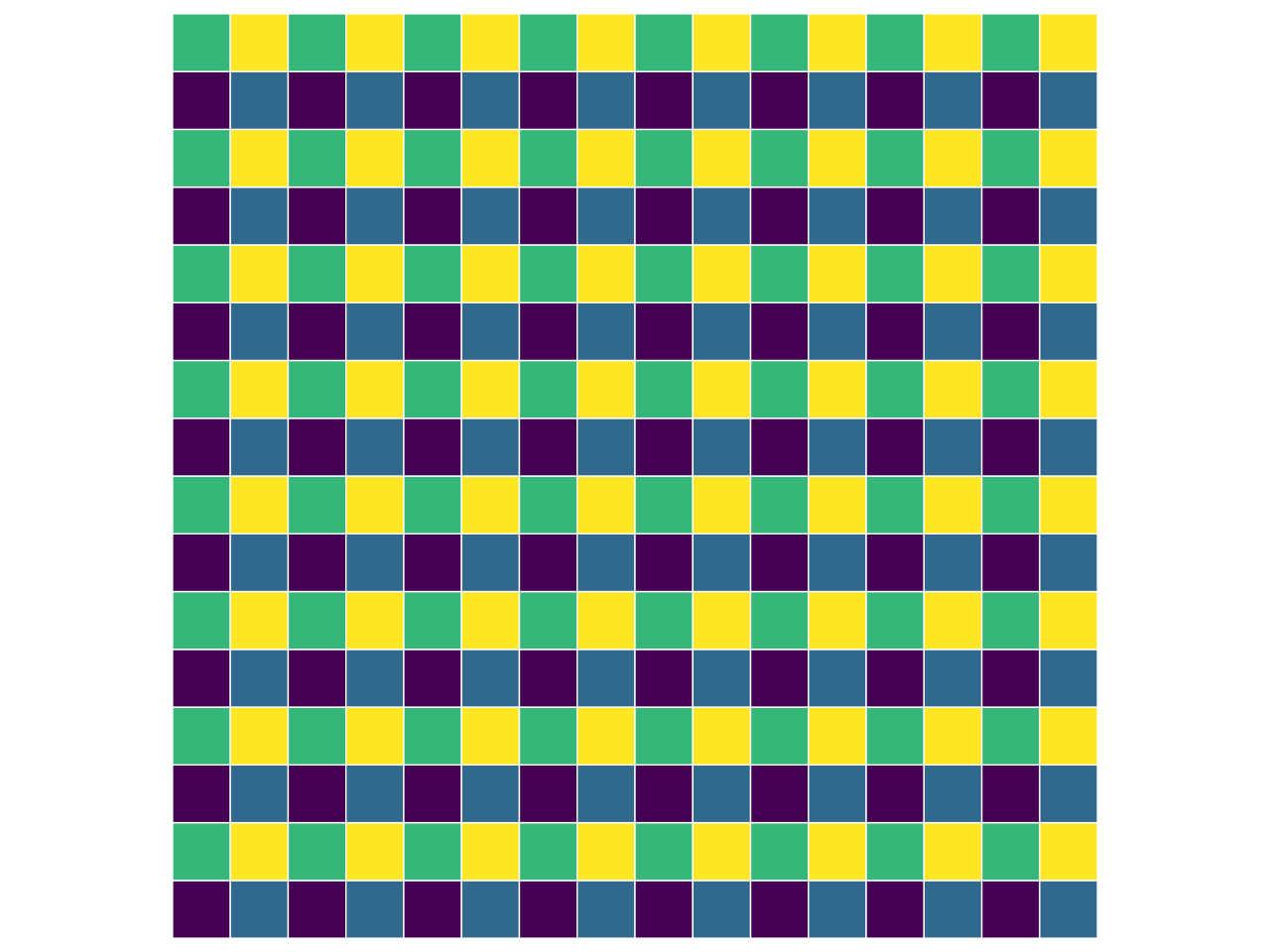

Figure 2: A 16x16 grid formed by repeating a 2x2 pattern.

# Let's demonstrate what it does
size = (2, 2)
repeat = (8, 8)

# Define a base 2x2 pattern
# base_pattern = torch.tensor([[0, 4, 8, 16], [1, 5, 9,] , [2], [3]], dtype=torch.float32)
base_pattern = np.arange(np.prod(size)).reshape(size)

base_pattern = torch.asarray(base_pattern)
base_pattern = base_pattern / base_pattern.numel()


# Repeat the pattern to get a 16x16 checkerboard
checkerboard = base_pattern.repeat(*repeat)
x = checkerboard.reshape(1, 1, *checkerboard.shape)

save_fig(show_image(x.numpy()), "checkerboard-input.webp")

p1, p2 = size
y = einops.rearrange(x, "b c (h p1) (w p2) -> b (c p1 p2) h w", p1=p1, p2=p2)
save_fig(show_image(y.numpy()), "checkerboard-rearranged.webp")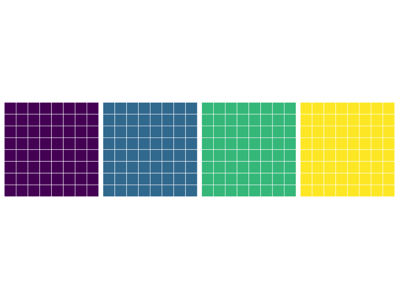

Figure 3: The four channels produced by moving each 2x2 neighborhood into the channel dimension.

Figure 2 and Figure 3 show only the rearrangement, before the learned convolution. The spatial dimensions halve and the channel count grows by 4x, with each new channel holding one position from every 2x2 window. Applying the inverse depth-to-space rearrangement at this point would recover the input exactly.

from einops.layers.torch import Rearrange


class RearrangePoolBlock(nn.Module):
    def __init__(self, in_chs: int, group_size: int) -> None:
        super().__init__()
        self.rearrange = Rearrange("b c (h p1) (w p2) -> b (c p1 p2) h w", p1=2, p2=2)
        self.conv = GELUConvBlock(4 * in_chs, in_chs, group_size)

    def forward(self, x: Tensor) -> Tensor:
        x = self.rearrange(x)
        return self.conv(x)

class DownBlock(nn.Module):
    def __init__(self, in_chs: int, out_chs: int, group_size: int) -> None:
        super().__init__()
        self.layers = nn.Sequential(
            GELUConvBlock(in_chs, out_chs, group_size),
            GELUConvBlock(out_chs, out_chs, group_size),
            RearrangePoolBlock(out_chs, group_size),
        )

    def forward(self, x: Tensor) -> Tensor:
        return self.layers(x)

class UpBlock(nn.Module):
    def __init__(self, in_chs: int, out_chs: int, group_size: int) -> None:
        super().__init__()
        self.layers = nn.Sequential(
            nn.ConvTranspose2d(2 * in_chs, out_chs, kernel_size=2, stride=2),
            GELUConvBlock(out_chs, out_chs, group_size),
            GELUConvBlock(out_chs, out_chs, group_size),
            GELUConvBlock(out_chs, out_chs, group_size),
            GELUConvBlock(out_chs, out_chs, group_size),
        )

    def forward(self, x: Tensor, skip: Tensor) -> Tensor:
        x = torch.cat((x, skip), 1)
        x = self.layers(x)
        return x

class ResidualConvBlock(nn.Module):
    def __init__(self, in_chs: int, out_chs: int, group_size: int) -> None:
        super().__init__()
        self.conv1 = GELUConvBlock(in_chs, out_chs, group_size)
        self.conv2 = GELUConvBlock(out_chs, out_chs, group_size)

    def forward(self, x: Tensor) -> Tensor:
        x1 = self.conv1(x)
        x2 = self.conv2(x1)
        out = x1 + x2
        return out

import math


class SinusoidalPositionEmbedBlock(nn.Module):
    def __init__(self, dim: int) -> None:
        super().__init__()
        self.dim = dim

    def forward(self, time: Tensor) -> Tensor:
        device = time.device
        half_dim = self.dim // 2
        embeddings = math.log(10_000) / (half_dim - 1)
        embeddings = torch.exp(torch.arange(half_dim, device=device) * -embeddings)
        embeddings = time[:, None] * embeddings[None, :]
        embeddings = torch.cat((embeddings.sin(), embeddings.cos()), dim=-1)
        return embeddings

class EmbedBlock(nn.Module):
    def __init__(self, input_dim: int, emb_dim: int) -> None:
        super().__init__()
        self.input_dim = input_dim
        self.model = nn.Sequential(
            nn.Linear(input_dim, emb_dim),
            nn.GELU(),
            nn.Linear(emb_dim, emb_dim),
            nn.Unflatten(1, (emb_dim, 1, 1)),
        )

    def forward(self, x: Tensor) -> Tensor:
        x = x.view(-1, self.input_dim)
        return self.model(x)

Putting the U-Net Together

The UNet forward pass has four details worth tracking:

• Timestep embeddings enter only the decoder. The encoder extracts features from the noisy image, and the decoder receives the noise-level signal at each resolution.
• The timestep embeddings are added to feature maps, which keeps the decoder channel counts unchanged.
• The last layer concatenates down0 with up2, carrying high-resolution features around the bottleneck.
• Despite their names, small_group_size and big_group_size are the numbers of GroupNorm groups. PyTorch requires that number to divide the channel count. The chosen values, 8 and 32, divide the relevant 64- and 128-channel layers.

class UNet(nn.Module):
    def __init__(self) -> None:
        super().__init__()
        img_chs = IMG_CH
        down_chs = (64, 64, 128)
        up_chs = down_chs[::-1]  # Reverse of the down channels
        latent_image_size = IMG_SIZE // 4  # 2 ** (len(down_chs) - 1)
        t_dim = 8
        group_size_base = 4
        small_group_size = 2 * group_size_base
        big_group_size = 8 * group_size_base

        # Initial convolution
        self.down0 = ResidualConvBlock(img_chs, down_chs[0], small_group_size)

        # Downsample
        self.down1 = DownBlock(down_chs[0], down_chs[1], big_group_size)
        self.down2 = DownBlock(down_chs[1], down_chs[2], big_group_size)
        self.to_vec = nn.Sequential(nn.Flatten(), nn.GELU())

        # Embeddings
        self.dense_emb = nn.Sequential(
            nn.Linear(down_chs[2] * latent_image_size**2, down_chs[1]),
            nn.ReLU(),
            nn.Linear(down_chs[1], down_chs[1]),
            nn.ReLU(),
            nn.Linear(down_chs[1], down_chs[2] * latent_image_size**2),
            nn.ReLU(),
        )

        # Time embeddings (temb)
        self.sinusoidaltime = SinusoidalPositionEmbedBlock(t_dim)
        self.temb_1 = EmbedBlock(t_dim, up_chs[0])
        self.temb_2 = EmbedBlock(t_dim, up_chs[1])

        # Upsample
        self.up0 = nn.Sequential(
            nn.Unflatten(1, (up_chs[0], latent_image_size, latent_image_size)),
            GELUConvBlock(up_chs[0], up_chs[0], big_group_size),
        )
        self.up1 = UpBlock(up_chs[0], up_chs[1], big_group_size)
        self.up2 = UpBlock(up_chs[1], up_chs[2], big_group_size)

        # Match output channels and one last concatenation
        self.out = nn.Sequential(
            nn.Conv2d(2 * up_chs[-1], up_chs[-1], 3, 1, 1),
            nn.GroupNorm(small_group_size, up_chs[-1]),
            nn.ReLU(),
            nn.Conv2d(up_chs[-1], img_chs, 3, 1, 1),
        )

    def forward(self, x: Tensor, t: Tensor) -> Tensor:
        down0 = self.down0(x)
        down1 = self.down1(down0)
        down2 = self.down2(down1)
        latent_vec = self.to_vec(down2)

        latent_vec = self.dense_emb(latent_vec)
        t = t.float() / T  # Convert from [0, T] to [0, 1]
        t = self.sinusoidaltime(t)

        up0 = self.up0(latent_vec)

        temb_1 = self.temb_1(t)
        up1 = self.up1(up0 + temb_1, down2)

        temb_2 = self.temb_2(t)
        up2 = self.up2(up1 + temb_2, down1)

        return self.out(torch.cat((up2, down0), 1))

model = UNet()
print("Num params: ", sum(p.numel() for p in model.parameters()))
model = torch.compile(model.to(device))

Num params:  1979777

import graphviz
from torchview import draw_graph

graphviz.set_jupyter_format("png")
model_graph = draw_graph(
    UNet(),
    input_size=((BATCH_SIZE, IMG_CH, IMG_SIZE, IMG_SIZE), (BATCH_SIZE,)),
    device="meta",
    depth=1,
    expand_nested=False,
    graph_dir="TD",
    graph_name="U-Net with Positional Embeddings",
)
model_graph.resize_graph(scale=0.75)
save_graph(model_graph.visual_graph, "unet-graph.webp")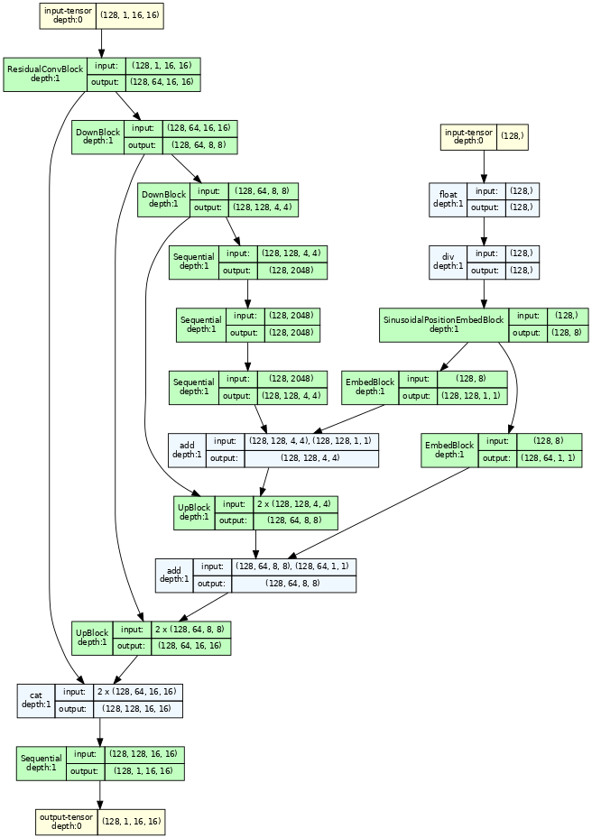

Figure 4: The U-Net backbone with timestep embeddings in the decoder.

Diffusion

A denoising diffusion probabilistic model (DDPM) learns to reverse a Markov chain that gradually adds Gaussian noise (Ho et al. 2020). Instead of producing an image in one pass, this implementation predicts the noise in \(x_t\) and applies that prediction repeatedly while moving from \(x_t\) toward \(x_{t-1}\).

Forward Process

For a conceptual index \(t=1,\ldots,T\), the forward transition is

\[ q(x_t \mid x_{t-1}) = \mathcal{N}\!\left(x_t; \sqrt{1-\beta_t}\,x_{t-1}, \beta_t\mathbf{I}\right). \]

Let \(\alpha_t=1-\beta_t\) and \(\bar{\alpha}_t=\prod_{s=1}^{t}\alpha_s\). Marginalizing the intermediate states gives

\[ q(x_t \mid x_0) = \mathcal{N}\!\left(x_t; \sqrt{\bar{\alpha}_t}\,x_0, (1-\bar{\alpha}_t)\mathbf{I}\right), \]

or, using \(\epsilon\sim\mathcal{N}(0,\mathbf{I})\),

\[ x_t = \sqrt{\bar{\alpha}_t}\,x_0 + \sqrt{1-\bar{\alpha}_t}\,\epsilon. \]

The code stores a_bar = torch.cumprod(a, dim=0). It can therefore sample any marginal \(q(x_t\mid x_0)\) directly. During training, it draws a separate timestep for every image in the batch.

Reverse Process

The network predicts \(\epsilon_\theta(x_t,t)\), and the implementation calculates

\[ \mu_\theta(x_t,t) = \frac{1}{\sqrt{\alpha_t}}\left(x_t - \frac{1-\alpha_t}{\sqrt{1-\bar{\alpha}_t}}\epsilon_\theta(x_t,t)\right). \]

For all but the last reverse step, it adds fresh Gaussian noise before continuing. The initial noise and these stochastic transitions allow different reverse trajectories.

This sampler is a simplified DDPM implementation. In particular, reverse_q() scales the added noise with the preceding schedule entry rather than the exact posterior variance derived in the DDPM formulation. The experiment therefore demonstrates the denoising mechanism, not an exact reproduction of the paper’s sampler.

def show_tensor_image(image):

    reverse_transforms = VT.Compose(
        [
            VT.Lambda(lambda t: (t + 1) / 2),
            VT.Lambda(lambda t: torch.minimum(torch.tensor([1]), t)),
            VT.Lambda(lambda t: torch.maximum(torch.tensor([0]), t)),
            VT.ToPILImage(),
        ]
    )
    plt.imshow(reverse_transforms(image[0].detach().cpu()))


class DDPM:
    def __init__(self, B: Tensor, device: torch.device) -> None:
        self.B = B
        self.T = len(B)
        self.device = device

        # Forward diffusion variables
        self.a = 1.0 - self.B
        self.a_bar = torch.cumprod(self.a, dim=0)
        self.sqrt_a_bar = torch.sqrt(self.a_bar)  # Mean Coefficient
        self.sqrt_one_minus_a_bar = torch.sqrt(1 - self.a_bar)  # St. Dev. Coefficient

        # Reverse diffusion variables
        self.sqrt_a_inv = torch.sqrt(1 / self.a)
        self.pred_noise_coeff = (1 - self.a) / torch.sqrt(1 - self.a_bar)

    def q(self, x_0: Tensor, t: Tensor) -> tuple[Tensor, Tensor]:
        """
        The forward diffusion process
        Returns the noise applied to an image at timestep t
        x_0: the original image
        t: timestep
        """
        t = t.int()
        noise = torch.randn_like(x_0)
        sqrt_a_bar_t = self.sqrt_a_bar[t, None, None, None]
        sqrt_one_minus_a_bar_t = self.sqrt_one_minus_a_bar[t, None, None, None]

        x_t = sqrt_a_bar_t * x_0 + sqrt_one_minus_a_bar_t * noise
        return x_t, noise

    def get_loss(self, model: nn.Module, x_0: Tensor, t: Tensor, *model_args: Tensor) -> Tensor:
        x_noisy, noise = self.q(x_0, t)
        noise_pred = model(x_noisy, t, *model_args)
        return F.mse_loss(noise, noise_pred)

    @torch.no_grad()
    def reverse_q(self, x_t: Tensor, t: Tensor, e_t: Tensor) -> Tensor:
        """
        The reverse diffusion process
        Returns an image with the noise from time t removed and time t-1 added.
        x_t: the noisy image at time t
        t: timestep
        e_t: the model's predicted noise at time t
        """
        t = t.int()
        pred_noise_coeff_t = self.pred_noise_coeff[t]
        sqrt_a_inv_t = self.sqrt_a_inv[t]
        u_t = sqrt_a_inv_t * (x_t - pred_noise_coeff_t * e_t)
        if t[0] == 0:  # All t values should be the same
            return u_t  # Reverse diffusion complete!
        else:
            B_t = self.B[t - 1]  # Apply noise from the previous timestep
            new_noise = torch.randn_like(x_t)
            return u_t + torch.sqrt(B_t) * new_noise

    @torch.no_grad()
    def sample_images(
        self, model: UNet, img_ch: int, img_size: int, ncols: int, *model_args: Tensor, axis_on: bool = False
    ) -> Figure:
        # Noise to generate images from
        x_t = torch.randn((1, img_ch, img_size, img_size), device=self.device)
        hidden_rows = self.T // ncols

        # Go from T to 0 removing and adding noise until t = 0
        imgs: list[np.ndarray] = []
        for i in reversed(range(self.T)):
            t = torch.full((1,), i, device=self.device).float()
            e_t = model(x_t, t, *model_args)  # Predicted noise
            x_t = self.reverse_q(x_t, t, e_t)
            if i % hidden_rows == 0:
                imgs.append(x_t.detach().squeeze().cpu().numpy())

        # A row of len(imgs) panels spans the 8-inch column, so the width is fixed and the
        # height is one panel's worth. Scaling height by the column count instead put this
        # figure past WebP's 16383 px limit once figures moved to 200 dpi.
        fig, axes = plt.subplots(ncols=len(imgs), figsize=(8, 8 / len(imgs)), frameon=False)
        for img, ax in zip(imgs, axes.flatten(), strict=True):
            ax.imshow(img, cmap="viridis", interpolation="none")
            ax.axis("on" if axis_on else "off")

        fig.tight_layout(pad=0.3)
        return fig

ddpm = DDPM(B, device)

Given \(x_0\), a timestep, and a sampled noise tensor, the closed-form forward calculation is deterministic. The panels in Figure 5 are independent samples from \(q(x_t\mid x_0)\): the code draws fresh noise for every panel instead of following one noise trajectory step by step.

set_random_seed()
idx = 0  # dataset index to visualize; change to try a different item/class
x0, _ = dataset[idx]
x0 = x0.unsqueeze(0).to(device)

x_ts = []
fig, axes = plt.subplots(nrows, ncols, figsize=(ncols, nrows), frameon=False)
for t_idx, ax in enumerate(axes.flat):
    t = torch.tensor([t_idx], device=device).float()
    x_t, _ = ddpm.q(x0, t)
    x_ts.append(x_t.squeeze().cpu().numpy())
    ax.imshow(x_ts[-1], cmap="viridis", interpolation="none", vmin=-1, vmax=1)
    ax.axis("off")

fig.tight_layout(pad=0.1)
save_fig(fig, "forward-diffusion.webp")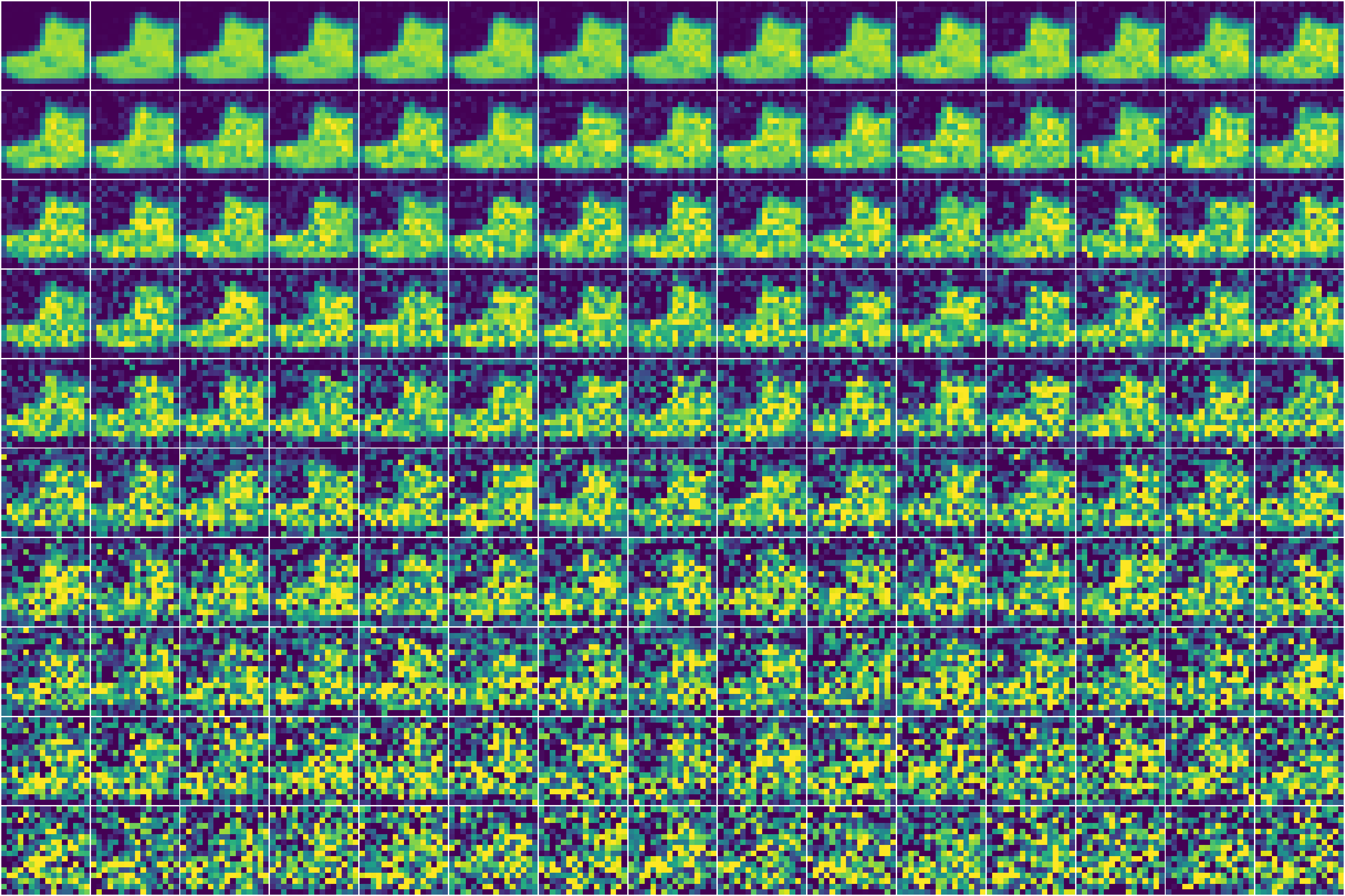

Figure 5: Independent samples from the forward marginal at timesteps 0 through 149, ordered from top left to bottom right.

Training Objective

The notebook uses the DDPM simplified objective: mean squared error between sampled noise \(\epsilon\) and predicted noise \(\epsilon_\theta(x_t,t)\) (Ho et al. 2020). Each update samples a timestep independently for every image, constructs \(x_t\) with the closed-form forward equation, predicts the noise, and backpropagates the error.

Five epochs are enough to show whether the loss decreases, but they are not a sample-quality benchmark. The stored log reports individual minibatch losses every 100 steps rather than epoch means, so its local fluctuations should not be interpreted as learning-curve reversals.

model = UNet().to(device)
model.compile()

optimizer = optim.Adam(model.parameters(), lr=0.001)
epochs = 5

model.train()
for epoch in range(epochs):
    for step, batch in enumerate(dataloader):
        optimizer.zero_grad()

        t = torch.randint(0, T, (BATCH_SIZE,), device=device).float()
        x = batch[0].to(device)
        loss = ddpm.get_loss(model, x, t)
        loss.backward()
        optimizer.step()

        if epoch % 2 == 0 and step % 100 == 0:
            name = f"samples-epoch-{epoch}-step-{step:03d}.webp"
            save_fig(ddpm.sample_images(model, IMG_CH, IMG_SIZE, ncols), name)
            print(f"Epoch {epoch} | step {step:03d} Loss: {loss.item()}")

Epoch 0 | step 000 Loss: 1.1058292388916016
Epoch 0 | step 100 Loss: 0.16490435600280762
Epoch 0 | step 200 Loss: 0.13419075310230255
Epoch 0 | step 300 Loss: 0.12638157606124878
Epoch 0 | step 400 Loss: 0.10222411155700684
Epoch 0 | step 500 Loss: 0.13434891402721405
Epoch 2 | step 000 Loss: 0.09219031035900116
Epoch 2 | step 100 Loss: 0.11431898921728134
Epoch 2 | step 200 Loss: 0.10901810228824615
Epoch 2 | step 300 Loss: 0.09168179333209991
Epoch 2 | step 400 Loss: 0.10279276967048645
Epoch 2 | step 500 Loss: 0.11188428848981857
Epoch 4 | step 000 Loss: 0.08083761483430862
Epoch 4 | step 100 Loss: 0.09731955081224442
Epoch 4 | step 200 Loss: 0.07860389351844788
Epoch 4 | step 300 Loss: 0.08876349776983261
Epoch 4 | step 400 Loss: 0.08546773344278336
Epoch 4 | step 500 Loss: 0.09255847334861755

Reverse trajectory after epoch 0, step 000.

Reverse trajectory after epoch 0, step 500.

Reverse trajectory after epoch 2, step 500.

Reverse trajectory after epoch 4, step 500.

In this run, the unconditional model’s saved reverse trajectories remain noisy. The final checkpoints contain broad garment-like regions, but I cannot identify a specific class reliably. Five epochs were not enough for this model and schedule to produce convincing unconditional samples.

The conditioned run below produces shapes that I find easier to recognize. It uses the same backbone and training budget, but it also adds class embeddings and starts from a separate random initialization. The contrast is useful as an observation, not controlled evidence that conditioning alone caused the difference.

Classifier-Free Guidance

Classifier-free guidance (CFG) trains one network to make both conditional and unconditional predictions, avoiding a separate classifier (Ho and Salimans 2022). During training, this notebook replaces the one-hot class vector with zeros with probability \(0.10\).

At inference, it evaluates both contexts and combines their noise predictions:

\[ \hat{\epsilon}_t = (1+w)\epsilon_\theta(x_t,t,c) - w\epsilon_\theta(x_t,t,\varnothing). \]

For this parameterization, \(w=0\) is the conditional prediction and \(w=-1\) is the unconditional prediction. Positive \(w\) extrapolates from the unconditional prediction toward the conditional one. Values below \(-1\) extrapolate in the opposite direction, but they do not guarantee a meaningful “not this class” sample. Every guided step costs two model evaluations.

From UNet to ContextUNet

ContextUNet retains the U-Net backbone and adds two learned class embeddings in the decoder. The class embedding scales each feature map while the timestep embedding shifts it:

up1 = self.up1(cemb_1 * up0 + temb_1, down2)

get_context() applies a Bernoulli mask to the one-hot class vector. A masked example enters the embedding network as a zero vector, allowing the same weights to learn the unconditional prediction used by CFG.

N_CLASSES = 10
DROP_PROB = 0.10


class ContextUNet(nn.Module):
    def __init__(self) -> None:
        super().__init__()
        img_chs = IMG_CH
        down_chs = (64, 64, 128)
        up_chs = down_chs[::-1]
        latent_image_size = IMG_SIZE // 4
        t_dim = 8
        group_size_base = 4
        small_group_size = 2 * group_size_base
        big_group_size = 8 * group_size_base

        self.down0 = ResidualConvBlock(img_chs, down_chs[0], small_group_size)
        self.down1 = DownBlock(down_chs[0], down_chs[1], big_group_size)
        self.down2 = DownBlock(down_chs[1], down_chs[2], big_group_size)
        self.to_vec = nn.Sequential(nn.Flatten(), nn.GELU())

        self.dense_emb = nn.Sequential(
            nn.Linear(down_chs[2] * latent_image_size**2, down_chs[1]),
            nn.ReLU(),
            nn.Linear(down_chs[1], down_chs[1]),
            nn.ReLU(),
            nn.Linear(down_chs[1], down_chs[2] * latent_image_size**2),
            nn.ReLU(),
        )

        self.sinusoidaltime = SinusoidalPositionEmbedBlock(t_dim)
        self.temb_1 = EmbedBlock(t_dim, up_chs[0])
        self.temb_2 = EmbedBlock(t_dim, up_chs[1])

        # Class context embeddings - parallel structure to time embeddings
        self.cemb_1 = EmbedBlock(N_CLASSES, up_chs[0])
        self.cemb_2 = EmbedBlock(N_CLASSES, up_chs[1])

        self.up0 = nn.Sequential(
            nn.Unflatten(1, (up_chs[0], latent_image_size, latent_image_size)),
            GELUConvBlock(up_chs[0], up_chs[0], big_group_size),
        )
        self.up1 = UpBlock(up_chs[0], up_chs[1], big_group_size)
        self.up2 = UpBlock(up_chs[1], up_chs[2], big_group_size)

        self.out = nn.Sequential(
            nn.Conv2d(2 * up_chs[-1], up_chs[-1], 3, 1, 1),
            nn.GroupNorm(small_group_size, up_chs[-1]),
            nn.ReLU(),
            nn.Conv2d(up_chs[-1], img_chs, 3, 1, 1),
        )

    def forward(self, x: Tensor, t: Tensor, c: Tensor) -> Tensor:
        down0 = self.down0(x)
        down1 = self.down1(down0)
        down2 = self.down2(down1)
        latent_vec = self.to_vec(down2)

        latent_vec = self.dense_emb(latent_vec)
        t = t.float() / T
        t = self.sinusoidaltime(t)

        up0 = self.up0(latent_vec)

        cemb_1 = self.cemb_1(c)
        temb_1 = self.temb_1(t)
        up1 = self.up1(cemb_1 * up0 + temb_1, down2)

        cemb_2 = self.cemb_2(c)
        temb_2 = self.temb_2(t)
        up2 = self.up2(cemb_2 * up1 + temb_2, down1)

        return self.out(torch.cat((up2, down0), 1))

graphviz.set_jupyter_format("png")
model_graph = draw_graph(
    ContextUNet(),
    input_size=(
        (BATCH_SIZE, IMG_CH, IMG_SIZE, IMG_SIZE),  # x
        (BATCH_SIZE,),  # t
        (BATCH_SIZE, N_CLASSES),  # c (class context)
    ),
    device="meta",
    depth=1,
    expand_nested=False,
    graph_dir="TD",
    graph_name="ContextUNet with Class Conditioning",
)
model_graph.resize_graph(scale=0.75)
save_graph(model_graph.visual_graph, "context-unet-graph.webp")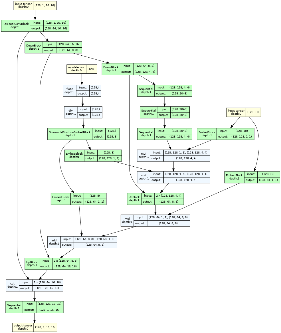

Figure 6: The conditioned U-Net with class and timestep embeddings in the decoder.

def get_context(labels: Tensor, drop_prob: float = DROP_PROB) -> Tensor:
    c_hot = F.one_hot(labels.to(torch.int64), num_classes=N_CLASSES).float()
    c_mask = torch.bernoulli(torch.ones(len(labels), device=labels.device) * (1 - drop_prob))
    return c_hot * c_mask[:, None]


context_model = ContextUNet().to(device)
context_model.compile()
optimizer = optim.Adam(context_model.parameters(), lr=0.001)
epochs = 5

context_model.train()
for epoch in range(epochs):
    for step, (x, labels) in enumerate(dataloader):
        optimizer.zero_grad()

        t = torch.randint(0, T, (BATCH_SIZE,), device=device).float()
        x = x.to(device)
        c = get_context(labels.to(device))

        loss = ddpm.get_loss(context_model, x, t, c)
        loss.backward()
        optimizer.step()

        if epoch % 2 == 0 and step % 100 == 0:
            print(f"Epoch {epoch} | step {step:03d} Loss: {loss.item():.4f}")

Epoch 0 | step 000 Loss: 1.0612
Epoch 0 | step 100 Loss: 0.1687
Epoch 0 | step 200 Loss: 0.1358
Epoch 0 | step 300 Loss: 0.1257
Epoch 0 | step 400 Loss: 0.0861
Epoch 0 | step 500 Loss: 0.1101
Epoch 2 | step 000 Loss: 0.0976
Epoch 2 | step 100 Loss: 0.0980
Epoch 2 | step 200 Loss: 0.0960
Epoch 2 | step 300 Loss: 0.0873
Epoch 2 | step 400 Loss: 0.0818
Epoch 2 | step 500 Loss: 0.0992
Epoch 4 | step 000 Loss: 0.0924
Epoch 4 | step 100 Loss: 0.0900
Epoch 4 | step 200 Loss: 0.0885
Epoch 4 | step 300 Loss: 0.1074
Epoch 4 | step 400 Loss: 0.0986
Epoch 4 | step 500 Loss: 0.0810

The stored conditional log falls from 1.0612 on its first recorded minibatch to 0.0810 on the last. The unconditional log moves from 1.1058 to 0.0926 at the corresponding recorded points. Both traces are noisy and broadly similar, so these values do not support the earlier claim that conditioning produced a smoother or faster loss descent. Sample inspection addresses a different question.

Interpreting the Guidance Weight

The implemented formula has several useful reference cases:

\(w\)	Prediction used
\(w < -1\)	Extrapolation away from the conditional prediction
\(w = -1\)	Unconditional prediction
\(-1 < w < 0\)	Interpolation between unconditional and conditional predictions
\(w = 0\)	Conditional prediction without extrapolation
\(w > 0\)	Extrapolation toward the conditional prediction

Larger positive weights often trade diversity for stronger conditioning, but an extreme value can also reduce sample quality (Ho and Salimans 2022). The single sample per grid cell below cannot measure either effect.

@torch.no_grad()
def sample_with_guidance(
    ddpm: DDPM,
    model: ContextUNet,
    class_label: int,
    w: float = 2.0,
) -> np.ndarray:
    x_t = torch.randn((1, IMG_CH, IMG_SIZE, IMG_SIZE), device=device)
    c = F.one_hot(torch.tensor([class_label], device=device), num_classes=N_CLASSES).float()
    c_empty = torch.zeros_like(c)

    for i in reversed(range(ddpm.T)):
        t = torch.full((1,), i, device=device).float()
        e_t_cond = model(x_t, t, c)
        e_t_uncond = model(x_t, t, c_empty)
        e_t = (1 + w) * e_t_cond - w * e_t_uncond
        x_t = ddpm.reverse_q(x_t, t, e_t)

    return x_t.squeeze().cpu().numpy()


fashion_classes = [
    "T-shirt",
    "Trousers",
    "Pullover",
    "Dress",
    "Coat",
    "Sandal",
    "Shirt",
    "Sneaker",
    "Bag",
    "Ankle boot",
]

fig, axes = plt.subplots(2, 5, figsize=(12, 5), constrained_layout=True)
for cls_idx, (ax, cls_name) in enumerate(zip(axes.flat, fashion_classes, strict=True)):
    img = sample_with_guidance(ddpm, context_model, cls_idx, w=2.0)
    ax.imshow(img, cmap="viridis", interpolation="none")
    ax.set_title(cls_name)
    ax.axis("off")
save_fig(fig, "class-conditioned-samples.webp")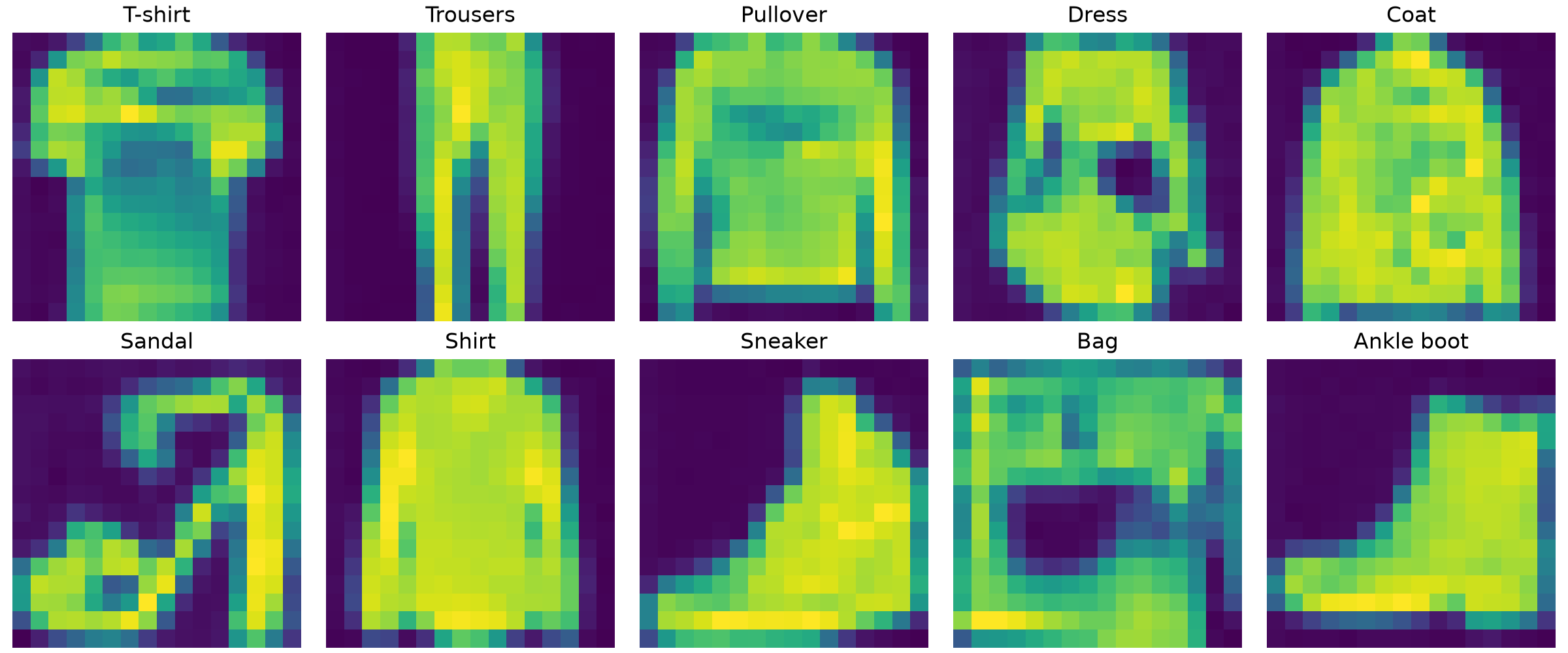

Figure 7: One generated sample for each FashionMNIST class at \(w=2\).

In Figure 7, I can associate most outputs with their requested class: trousers have separate legs, while the sneaker and ankle boot have distinct profiles. This is one sample per class from one trained model, so it is a qualitative check rather than an accuracy result. The sweep below varies \(w\) while keeping the class labels fixed.

w_values = [-2.0, 0.0, 1.0, 2.0, 5.0]
selected_classes = [0, 1, 7, 9]  # T-shirt, Trousers, Sneaker, Ankle boot

fig, axes = plt.subplots(len(w_values), len(selected_classes), figsize=(8, 10), constrained_layout=True)
for row, w in enumerate(w_values):
    for col, cls_idx in enumerate(selected_classes):
        img = sample_with_guidance(ddpm, context_model, cls_idx, w=w)
        ax = axes[row, col]
        ax.imshow(img, cmap="viridis", interpolation="none")
        ax.axis("off")
        if row == 0:
            ax.set_title(fashion_classes[cls_idx], fontsize=9)
        if col == 0:
            ax.set_ylabel(f"w={w}", rotation=0, labelpad=35, va="center")

fig.suptitle("Guidance weight (rows) × class (columns)", y=1.01)
save_fig(fig, "guidance-weight-sweep.webp")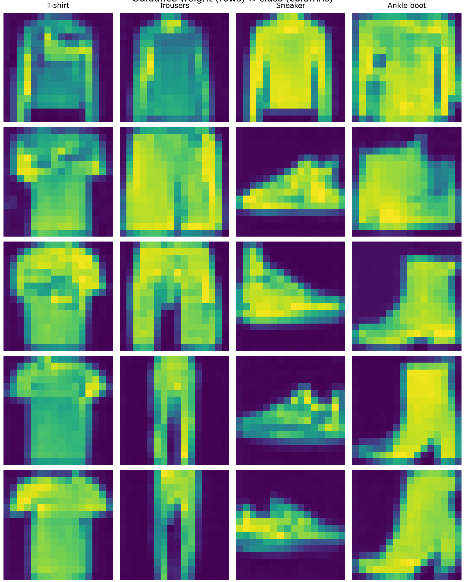

Figure 8: One generated sample for four classes at each tested guidance weight.

I expected \(w=-2\) to produce recognizable alternatives to the requested classes. In Figure 8 it mostly produces rougher shapes, which is consistent with extrapolating away from the conditional prediction but does not amount to semantic anti-guidance. Changes from \(w=0\) through \(w=5\) are also modest in these particular samples. Because every cell uses one random draw, the grid cannot separate a systematic guidance effect from seed variation.

Conclusion

Three implementation details changed how I read this experiment. First, the cumulative product \(\bar{\alpha}_t\) makes random-timestep training practical by sampling \(x_t\) directly. Second, space-to-depth is lossless only before its learned channel compression, and it is separate from the transposed-convolution overlap that can create checkerboards. Third, the CFG weight must be interpreted from the exact blending formula: in this notebook, \(w=0\) is conditional and \(w=-1\) is unconditional.

The generated images suggest that the conditioned model learned more recognizable shapes within this five-epoch budget, while the recorded minibatch losses do not show a clear optimization advantage. Repeated runs, more samples per class, and a schedule whose endpoint is closer to Gaussian noise would be needed before drawing a broader performance conclusion.

For a more theoretical treatment, Lilian Weng’s What Are Diffusion Models? connects DDPMs with score matching and stochastic differential equations.

References

Hendrycks, Dan, and Kevin Gimpel. 2016. “Gaussian Error Linear Units (GELUs).” arXiv Preprint arXiv:1606.08415. https://arxiv.org/abs/1606.08415.

Ho, Jonathan, Ajay Jain, and Pieter Abbeel. 2020. “Denoising Diffusion Probabilistic Models.” Advances in Neural Information Processing Systems 33: 6840–51. https://proceedings.neurips.cc/paper/2020/hash/4c5bcfec8584af0d967f1ab10179ca4b-Abstract.html.

Ho, Jonathan, and Tim Salimans. 2022. “Classifier-Free Diffusion Guidance.” arXiv Preprint arXiv:2207.12598. https://arxiv.org/abs/2207.12598.

Odena, Augustus, Vincent Dumoulin, and Chris Olah. 2016. “Deconvolution and Checkerboard Artifacts.” Distill, ahead of print. https://doi.org/10.23915/distill.00003.

Ronneberger, Olaf, Philipp Fischer, and Thomas Brox. 2015. “U-Net: Convolutional Networks for Biomedical Image Segmentation.” Medical Image Computing and Computer-Assisted Intervention – MICCAI 2015, 234–41. https://doi.org/10.1007/978-3-319-24574-4_28.

Vaswani, Ashish, Noam Shazeer, Niki Parmar, et al. 2017. “Attention Is All You Need.” Advances in Neural Information Processing Systems 30: 5998–6008.

Wu, Yuxin, and Kaiming He. 2018. “Group Normalization.” European Conference on Computer Vision (ECCV), 3–19. https://doi.org/10.1007/978-3-030-01261-8_1.