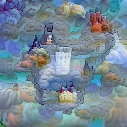
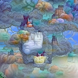
CLIP can score how well an image matches a text prompt, but on its own it has no way to produce one. VQGAN+CLIP closes that gap by optimizing a latent vector fed through a pretrained VQGAN decoder, descending a loss that measures how far the decoded image’s CLIP embedding sits from the prompt’s. The decoder supplies a learned prior over realistic image structure, so optimization changes the latent that generates the image rather than pixels directly.
Introduction
In 2021, I came across one of the early VQGAN+CLIP notebooks, and it surprised me: dreamy, surrealistic images that felt like their own branch of art, pulled out of nothing but a line of text. I didn’t have time to dig into it then, so I filed it away and moved on to other things.
DALL-E, Midjourney, and Stable Diffusion then left the approach behind, but the notebook kept surfacing in my Colab history. This post is the overdue look at how it actually worked.
The mechanism is small enough to state up front. VQGAN supplies a generator and CLIP supplies a judge; both stay frozen, and the only thing that ever changes is the generator’s input. Adam descends a loss measuring how far the decoded image’s CLIP embedding sits from the prompt’s, and no network is trained anywhere.
That loop alone is enough to produce recognizable images: what’s now called text-to-image generation. First, though, it helps to see where VQGAN+CLIP sits in that timeline.
Where VQGAN+CLIP Sits in History
VQGAN+CLIP was short-lived (CLIP-guided diffusion displaced it within about a year), but it sits at an important hinge point: the bridge between old GAN1-era image synthesis and the text-to-image diffusion models that followed.
The immediate precursor was BigGAN+CLIP, best known through advadnoun’s Big Sleep3. CLIP’s weights were released in January 2021, and Big Sleep was one of the first systems built on them (Oppenlaender 2023). A pretrained BigGAN supplied the generator, and CLIP guided a class-conditioned latent vector toward a text prompt by gradient ascent: the same “frozen generator, frozen scorer, optimize the input” idea this post uses, just with a different generator.
BigGAN’s prior was narrow: trained on ImageNet, it “wanted” to draw ImageNet-like objects, with a latent that was just one global vector plus a class label. VQGAN’s latent is a spatial grid of image tokens instead (Esser et al. 2021), a much less constrained prior. Katherine Crowson connected it to CLIP next, formalized the following year as the VQGAN-CLIP paper (Crowson et al. 2022). By most accounts, that looser prior is why VQGAN+CLIP could push open-ended prompts (landscapes, architecture, surreal compositions) further than BigGAN+CLIP’s narrower, object-centric one ever could.
The mechanism was hacky and it was superseded fast, once diffusion models learned text conditioning directly instead of needing it bolted on after the fact. Neither fact makes it a failed branch: it mattered historically and artistically, and what the supersession looked like is covered in the Appendix. With the context set, here’s how the two components work.
VQGAN
Think of a generator network as a sculptor working with a fixed repertoire of chisel strokes: it can combine those strokes in many ways, but it cannot work independently of what it has learned. A VQGAN4, introduced in the Taming Transformers paper (Esser et al. 2021), uses an autoencoder whose decoder reconstructs images from a compressed, discrete codebook. The codebook constrains its outputs to visual structures represented by those learned codes.
Formally, a VQGAN has three parts: an encoder that maps an image down to a small spatial grid of continuous vectors, a quantizer that snaps each vector to its nearest entry in a learned codebook, and a decoder that turns the quantized grid back into a full-resolution image. Only the quantizer and decoder matter here: nothing in this post trains a new VQGAN, and nothing needs the encoder.
The checkpoint used here is the vqvae component of a latent-diffusion model trained on OpenImages: it downsamples 4x in each dimension with an 8192-entry codebook, so a 32x32x3 latent decodes to a 128x128 image. The decoder was trained at a native resolution of 256x256 (sample_size=256). The flagship demo later in this post reaches for that native size instead of the smaller default.
The decoder constrains each output to combinations of patterns represented by its codebook. Optimization can steer which patterns appear and how they are composed, but it remains within that learned representation.
def load_vqgan( device: torch.device, model_id: str="CompVis/ldm-super-resolution-4x-openimages",) -> VQModel:# CRITICAL, not ERROR: diffusers logs the "no safetensors file, falling back to .bin"# notice at ERROR level even though the load succeeds.for logger_name in ("diffusers", "huggingface_hub"): logging.getLogger(logger_name).setLevel(logging.CRITICAL)with warnings.catch_warnings(): warnings.simplefilter("ignore", category=UserWarning) vqgan = VQModel.from_pretrained(model_id, subfolder="vqvae").to(device) vqgan.eval() vqgan.requires_grad_(False)return vqganvqgan = load_vqgan(device=device)downsample_factor =2** (len(vqgan.config.block_out_channels) -1)print(f"Codebook size: {vqgan.config.num_vq_embeddings}")print(f"Latent channels: {vqgan.config.latent_channels}")print(f"Downsampling factor: {downsample_factor}x")
With the generator covered, the other half of VQGAN+CLIP is the judge that scores its output. CLIP5 is used here purely as a scorer: nothing about it gets fine-tuned, and it never conditions a generator during training. It grades a generator’s output after the fact, and the optimizer chases that grade.
Formally, CLIP exposes two encoders that map into the same 512-dimensional space: an image encoder and a text encoder. Cosine similarity between an image embedding and a text embedding measures how well the two match: high similarity means related content, low similarity means unrelated.
clip.load(...) returns the model in fp16 on CUDA by default, fine for frozen inference. The reference notebooks all switch to fp32 with .float() before backpropagating through CLIP, on the reasoning that fp16’s narrow dynamic range makes gradients unstable. Testing that directly (600 iterations, same prompt and seed as the flagship run, fp16 vs. bf16 vs. fp32) turned up no NaN or Inf gradients in any of the three. Final CLIP similarity landed within 0.01 across all of them, fp32 only slightly ahead. So .float() here is a precaution carried over from the community notebooks rather than something this specific setup demonstrates is required. It’s kept as the default anyway: fp32 is the safest option, and the VQGAN decoder’s own forward+backward pass dominates the per-iteration cost regardless of what precision CLIP runs at.
CLIP also has its own normalization statistics, different from the ImageNet mean/std reused in Neural Style Transfer and Feature Maps. Reusing the wrong constants here would silently corrupt every gradient CLIP produces.
Every post so far that trained something did it by adjusting a network’s weights. This one adjusts none: CLIP and the VQGAN decoder are both frozen for the entire run. So what does the optimizer push on?
Instead of optimizing pixels, Adam can optimize a point in the decoder’s input space.
Formally, the setup is:
Encode the target prompt once with CLIP’s text encoder into a single fixed 512-dim vector: the goal the whole run pushes toward.
Initialize a latent z of shape (1, 3, 32, 32) as random noise, with requires_grad=True. This is the only trainable tensor in the entire process.
Decode z into an image, score that image against the goal, and backpropagate through CLIP, through the decoder, all the way back to z.
Take an Adam step on z alone.
Step 3 hides one subtlety. The quantizer snaps each latent vector to its nearest codebook entry, and a nearest-neighbor lookup is piecewise constant: its derivative is zero almost everywhere, so it passes no useful gradient. Quantized VQ models get around this with a straight-through estimator, z_q = z + (z_q - z).detach(), which hands the decoder’s incoming gradient back to the pre-quantization vector unchanged. diffusers’ VectorQuantizer does exactly this, and it is the only reason gradients reach z at all with quantize=True.
The diagram below traces exactly where gradients flow versus where they stop:
flowchart LR
    subgraph Trainable
        z[("z<br/>latent (1,3,32,32)")]
    end
    subgraph "Frozen VQGAN"
        vq["quantize + decode"]
    end
    img["image<br/>(1,3,128,128)"]
    cut["make_cutouts<br/>x32"]
    subgraph "Frozen CLIP"
        cimg["image encoder"]
        ctxt["text encoder"]
    end
    embi["image embeddings<br/>(32,512)"]
    embt["text embedding<br/>(1,512)"]
    prompt(["text prompt"])
    dist["spherical distance<br/>(mean over 32 cutouts)"]
    loss["loss = mean(dist)"]

    z --> vq --> img --> cut --> cimg --> embi
    prompt --> ctxt --> embt
    embi --> dist
    embt --> dist
    dist --> loss
    loss -. "backward(): gradient passes through cimg, cut, vq" .-> z

    classDef frozen fill:#eee,stroke:#999,color:#555
    class vq,cimg,ctxt frozen
Gradient flows from the CLIP similarity loss back through frozen CLIP and the frozen VQGAN decoder, but only the latent z ever gets updated. Shapes and counts are the defaults; the flagship run below uses a 64x64 latent and 64 cutouts.
@dataclassclass HallucinationConfig: prompt: str latent_size: int=32 latent_channels: int=3 n_iters: int=400 cutn: int=32# number of random crops scored per iteration, see "Why 32 Crops Instead of One" cut_pow: float=1.0 cut_size: int=224 lr: float=0.1 quantize: bool=True seed: int= SEED snapshot_every: int=1 loss_fn: Literal["cosine", "spherical"] ="spherical"# see "Scoring and Climbing" and the appendix
Why 32 Crops Instead of One
A single, fixed 224x224 view of the decoded image gives Adam exactly one thing to satisfy. It’s entirely possible to nudge z toward a decoded image that scores well from that one framing but looks like nothing in particular from any other angle. That’s the classic adversarial-example failure mode, just happening inside a latent instead of directly in pixel space.
The fix used by every VQGAN+CLIP implementation, including the community reference notebooks covered in the Appendix: score many independently random crops of the same image and average the result. A change that raises the average similarity over dozens of random crop positions, sizes, and flips has to be visible in the image, not just exploitable from one exact viewpoint.
One view is a peephole; many random ones force a consensus.
The choice of 32 follows the reference notebooks’ convention rather than any principled derivation.
Note
The reference notebooks use kornia.augmentation for this specifically because it can sample an independent random transform per item within a single batched call (same_on_batch=False). torchvision’s batched transforms, by contrast, sample one shared transform for the whole batch. At this notebook’s scale (32 cutouts of a 128x128 image), a plain Python loop calling per-cutout crop and resize operations is negligible overhead, and it avoids adding a dependency (kornia) that isn’t used anywhere else in this blog.
The crop count isn’t free of scale, either. In my runs, bumping the canvas from 128x128 to the decoder’s native 256x256 while leaving cutn at 32 let a faint adversarial texture creep back in: a repeating high-frequency pattern spread across the image, with the similarity score climbing as it emerged. Doubling cutn to 64 removed it, which is why the flagship demo below raises both together: more area to cover needs more independent glances at it.
Each cutout gets its own CLIP image embedding, and cosine similarity against the fixed text embedding gives one score per cutout: the higher the similarity, the smaller the angle \(\theta_i\) between cutout \(i\)’s embedding and the text embedding. The loss is the mean spherical distance over all \(N\) cutouts (cutn), Katherine Crowson’s formulation:
That’s algebraically just \(\frac{1}{N}\sum_{i=1}^{N} \frac{\theta_i^2}{2}\), the mean spherical distance between each cutout embedding and the text embedding. It’s computed this way, through the embedding difference, rather than more directly as \(\arccos(\cos\theta_i)\): both give the identical value, but arcsin’s gradient stays well-behaved as \(\theta \to 0\) while \(\arccos\)’s blows up there, a likely reason Crowson’s original formula avoids it.
Minimizing \(\mathcal{L}\) still drives cosine similarity up, but not by the route a plain \(\mathcal{L}_{\cos}(z) = -\frac{1}{N}\sum_{i=1}^{N}\cos\theta_i\) loss would take: cosine similarity’s gradient fades out for badly-mismatched crops right when a stronger correction is needed, while spherical distance’s keeps growing with the angle. The Appendix works through that argument, and through why this post’s measurement doesn’t settle it.
Unlike Neural Style Transfer, this implementation has no total-variation (TV) loss. There, TV discourages high-frequency artifacts that direct pixel optimization can exploit. Here, optimization acts through a pretrained decoder rather than independent pixels, and the resulting images stayed spatially coherent in these runs. I therefore leave TV out; adding it would introduce a smoothness-detail tradeoff that this experiment did not need.
def hallucinate( cfg: HallucinationConfig, vqgan: VQModel, clip_model: torch.nn.Module, device: torch.device,) ->tuple[Tensor, list[np.ndarray], float]: torch.manual_seed(cfg.seed) z = torch.randn(1, cfg.latent_channels, cfg.latent_size, cfg.latent_size, device=device, requires_grad=True) optimizer = optim.Adam([z], lr=cfg.lr) tokens = clip.tokenize([cfg.prompt]).to(device)with torch.no_grad(): text_emb = clip_model.encode_text(tokens).float() text_emb = text_emb / text_emb.norm(dim=-1, keepdim=True) snapshots = [] pbar = tqdm(range(cfg.n_iters))for i in pbar: img = latent_to_image(vqgan, z, cfg.quantize) cutouts = make_cutouts(img, cfg.cutn, cfg.cut_size, cfg.cut_pow) img_emb = clip_model.encode_image(cutouts) img_emb = img_emb / img_emb.norm(dim=-1, keepdim=True)# Cosine similarity is tracked either way: it's the comparable metric across both# loss functions, not just the cosine-loss objective itself. similarity = (img_emb * text_emb).sum(dim=-1).mean()if cfg.loss_fn =="spherical": dists = img_emb.sub(text_emb).norm(dim=-1).div(2).arcsin().pow(2).mul(2) loss = dists.mean()else: loss =-similarity optimizer.zero_grad() loss.backward() optimizer.step() pbar.set_postfix_str(f"loss={loss.item():.4f} similarity={similarity.item():.4f}")if i % cfg.snapshot_every ==0or i == cfg.n_iters -1:with torch.no_grad(): snapshot = latent_to_image(vqgan, z, cfg.quantize) snapshots.append(snapshot.squeeze(0).permute(1, 2, 0).cpu().numpy())with torch.no_grad(): final_image = latent_to_image(vqgan, z, cfg.quantize).squeeze(0)return final_image, snapshots, similarity.item()
def log_spaced_indices(n_frames: int, ncols: int) -> np.ndarray:"""Frame indices weighted toward the start, where the image changes fastest."""if n_frames <= ncols:return np.arange(n_frames) indices = np.unique(np.r_[0, np.geomspace(1, n_frames -1, num=ncols -1).round().astype(int)]) unused = np.setdiff1d(np.arange(n_frames), indices)return np.sort(np.r_[indices, unused[: ncols -len(indices)]])def save_progression(frames: list[np.ndarray], name: str, ncols: int=8) ->list[int]:"""Write a log-spaced filmstrip of the run to figures/ and return the iterations shown.""" indices = log_spaced_indices(len(frames), min(len(frames), ncols)) save_webp(filmstrip([frames[i] for i in indices]), name)return indices.tolist()
Hallucinating from Noise
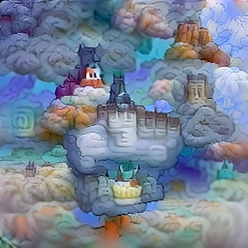
Everything is in place. This flagship run starts z from random noise and pushes it toward “a castle in the clouds,” snapshotting the decoded image every iteration. That makes it possible to inspect the run two ways: as a handful of evenly-spaced stills here, and as a full video next.
It overrides three defaults: latent_size=64 (the decoder’s native 256x256 resolution), cutn=64 (the doubled crop count that keeps it clean at that size, per the previous section), and n_iters=600. The extra 200 iterations are margin rather than necessity: the similarity score had plateaued well before the end in my runs, and the tail of the run only refines texture. That costs about 120 seconds against 30 for a default run, worth it for the one hero image and video but not for every generation in this post. The eight stills below are spaced logarithmically rather than evenly, because the run converges far faster than it finishes: the jump from noise to a recognizable castle happens within the first few dozen iterations, and everything after that is refinement. Each panel is labelled with its iteration number.
set_random_seed()cfg = HallucinationConfig(prompt="a castle in the clouds", latent_size=64, cutn=64, n_iters=600)final_image, snapshots, similarity_flagship = hallucinate(cfg, vqgan, clip_model, device)progression_iters = save_progression(snapshots, "flagship-progression.webp")print(f"Flagship final similarity: {similarity_flagship:.4f}")print(f"Filmstrip iterations: {progression_iters}")
Iterations 0, 1, 3, 8, 24, 71, 206 and 599 of “a castle in the clouds”, left to right. A recognizable castle appears within the first few dozen steps; everything after that is refinement.
Watching It Hallucinate
The stills above sample only eight of the 600 iterations. The full sequence of per-iteration snapshots can become a short video instead, one frame per iteration.
A 256x256 video still looks small blown up on a modern screen, though. To see exactly what “blown up” means here, the cell below stretches the flagship image to 512x512 with Lanczos resampling (a sharper classical filter than bicubic, but still no model involved):
The flagship image, 256x256 stretched to 512x512 with Lanczos resampling and no model involved.
Soft and a little muddy: stretching pixels doesn’t invent detail that was never decoded in the first place. At such a modest factor, though, that softness is barely worth fixing: 256x256 to 512x512 is only 2x, and the VQGAN decoder’s own painterly, texture-heavy look already hides most of it. A learned upscaler like Swin2SR would sharpen things further, but adding one means an extra frozen forward pass over every frame for a gain that isn’t worth the added complexity at this scale. The video below uses this same Lanczos resize on every frame: no model, no extra dependency.
A Small Gallery
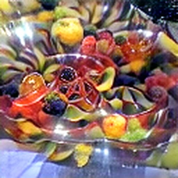
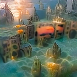
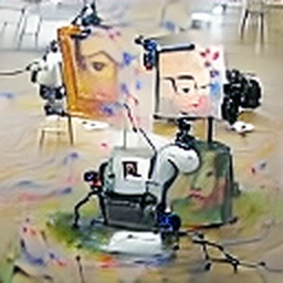
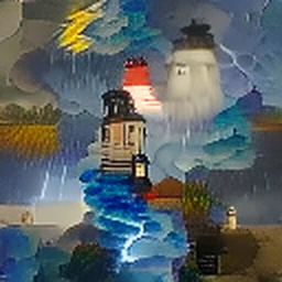
A few more prompts, run independently through the same hallucinate() function above: nothing changes except the prompt. Every run reuses the same seed, so all four start from the identical random latent and any difference between them comes from the prompt alone.
gallery_prompts = ["a bowl of fruit made of glass","an underwater city at sunset","a robot painting a self-portrait","a lighthouse in a thunderstorm",]for index, prompt inenumerate(gallery_prompts, start=1): set_random_seed() cfg = HallucinationConfig(prompt=prompt) img, _, _ = hallucinate(cfg, vqgan, clip_model, device) upscaled = upscale_lanczos(img.permute(1, 2, 0).cpu().numpy(), (256, 256)) save_webp(upscaled, f"gallery-{index}.webp")
The images above share a recognizable aesthetic: painterly and texture-rich, symbolic rather than exact, often striking in one region and incoherent across the whole. This comes directly from the random-cutout scoring explained in “Why 32 Crops Instead of One” above: CLIP only ever judges small crops, so the optimizer scatters many locally prompt-related textures across the canvas rather than composing one coherent global scene.
VQGAN+CLIP doesn’t paint a scene: it collages together whatever textures CLIP recognizes as matching the prompt.
This is the same dreamlike quality that caught my eye back in 2021. Now I know where it comes from.
Takeaways
No training, no dataset, one GPU, and about 30 seconds an image at the defaults: that is the whole cost of turning a pretrained decoder and a pretrained scorer into a text-to-image generator. That it works at all is the headline. What I actually learned is where it stops working.
Regularization barely matters here, right until it does. There is no total-variation term or octave schedule because the pretrained decoder already constrains outputs to its learned representation. But the crop count turned out to be regularization wearing a different hat, and it quietly stopped doing its job the moment I changed resolution and nothing else. Any safeguard that works by sampling the image is tied to how large that image is, and nothing warns you when the sampling gets too thin.
The loss function mattered less than the theory led me to expect, and I only found that out by rerunning. Crowson’s spherical distance has the better gradient shape on paper. An earlier run had it ahead of negative cosine similarity by 0.0014; rerunning the identical cells put it 0.0128 behind, and a third run 0.0032 behind. The ordering isn’t stable, so the experiment never had the resolution to answer the question I was asking it. Spherical distance stays the default because every reference implementation uses it, not because this comparison earned it. The Appendix has the derivation and the full account.
What didn’t work as well, in prompts tried beyond the four shown in the gallery above: concepts far outside what an OpenImages-trained decoder has textures for tend to converge to a generic, blurry approximation rather than anything specific. Call it a “vocabulary ceiling.” Literal, compositional prompts (several distinct named objects in a specific arrangement) also tend to blend together rather than stay separated, a consequence of scoring one pooled cosine similarity rather than anything spatially localized.
Appendix
Provenance of the Reference Notebooks
The four community reference notebooks used while testing this post all trace back to the same lineage: advadnoun’s original BigGAN+CLIP approach, followed by Katherine Crowson’s VQGAN+CLIP “z+quantize” notebook. From there the family splits. nerdyrodent ported the Colab notebook to a local command-line tool. dribnet’s clipit package forked nerdyrodent’s version and, per its own README, “quickly morphed into its own tuned version.” Chigozie Nri built a separate zoom/pan/keyframe animation notebook on the same base (chigozienri/VQGAN-CLIP-animations).
Justin John maintains a collection of these variants at justinjohn0306/VQGAN-CLIP, including two of the four reference notebooks used here, VQGAN+CLIP(Updated).ipynb and VQGAN+CLIP_(Zooming)_(z+quantize_method_with_addons).ipynb, both created within days of each other in August 2021 per that repo’s commit history. A third, VQGAN+CLIP (with overlays).ipynb, isn’t in that repo: it wraps dribnet’s clipit package directly, and now lives in dribnet/clipit’s demos/ folder under the filename Moar_Settings.ipynb (its embedded Colab title still reads “with overlays”). Its own credits point to the fourth: a Spanish-language translation and extension of Crowson’s original notebook by Eleiber#8347 and Abulafia#3734, hosted on Colab (the same notebook linked in the Introduction), a parallel branch I couldn’t date as precisely.
The community kept extending VQGAN+CLIP for a while before diffusion took over.
Scaling attempts stayed hacky: people pushed to larger canvases (512x512, 768x512, and up), but VQGAN’s latent is spatial, so a bigger output means a bigger latent grid and slower, less stable optimization. That’s exactly the tiling artifact this post ran into in the 512x512 dead end below. Higher-resolution runs also tended toward “detail soup”: the same crop-level myopia described in “The VQGAN+CLIP Look” above, and worse the more canvas there is to fill. Zoom-and-pan “infinite canvas” videos and init-image workflows (start from a real photo instead of noise) were the other big extensions. The community’s actual answer for “bigger and sharper” was almost always generate-then-upscale: the same split this post lands on.
Beyond scaling, the underlying pattern itself kept generalizing too. Pixray6, created by Tom White (dribnet) in September 2021, folded it into one tool: the same prompt-vs-CLIP-similarity objective, but with a swappable “drawer”: raw pixels, a VQGAN latent, vector strokes (CLIPDraw), or other representations. It credits Perception Engines, the CLIP-guided GAN work of advadnoun and Crowson, and CLIPDraw as direct ancestors.
The real successor to the “optimize an image against CLIP every time” family was CLIP-guided diffusion: guiding a diffusion model’s sampling with CLIP gradients instead of optimizing a VQGAN latent or raw pixels. Crowson’s CLIP-guided diffusion notebook became the basis for Disco Diffusion (popularized in November 2021), slower and dreamlike, but more coherent than raw VQGAN+CLIP. After that, the field moved toward models trained end-to-end for text conditioning (Stable Diffusion and contemporaries), and CLIP shifted from being the entire conditioning mechanism to one signal among several.
That generate-then-upscale split relied on whatever upscaling tools existed at the time. A learned upscaler like Swin2SR didn’t exist when these reference notebooks were written. Real-ESRGAN (arXiv 2021-07) and SwinIR (arXiv 2021-08) were both released within a month of the reference notebooks, which is why chaining a Real-ESRGAN pass after generation became common practice in that community. Swin2SR wasn’t published until 2022-09, over a year later, and would have been the natural hindsight pick for this notebook’s post-processing step, since transformers is already a dependency here. It went unused for the reason given in “Watching It Hallucinate” above: at 2x, plain Lanczos was enough.
Another Idea Tried From These Notebooks: Codebook-Based z Init
The reference notebooks initialize z from a random combination of actual codebook embedding vectors (one_hot @ quantize.embedding.weight) rather than torch.randn, on the theory that starting inside the codebook’s value range gives cleaner early gradients. I swapped it in, matching the seed and everything else, and saw no meaningful difference: a ~0.005-0.008 edge for codebook init in the first 20 iterations (within run-to-run noise), and torch.randn slightly ahead again by iteration 600 (0.5056 vs. 0.5014). Compute cost was identical. The checkpoint’s embedding statistics explain why: mean ~0.02, std ~0.65, not far from a standard Gaussian, so there’s no “wrong neighborhood” problem for torch.randn to fix.
Another Idea Tried: Generating Directly at 512x512
Rather than generating at 256x256 and upscaling afterward, the cell below runs the same hallucinate() pipeline directly at latent_size=128 (512x512 with this decoder’s 4x downsampling). It uses the same prompt and seed as the flagship run, with cutn=128: no upscaling anywhere in the loop.
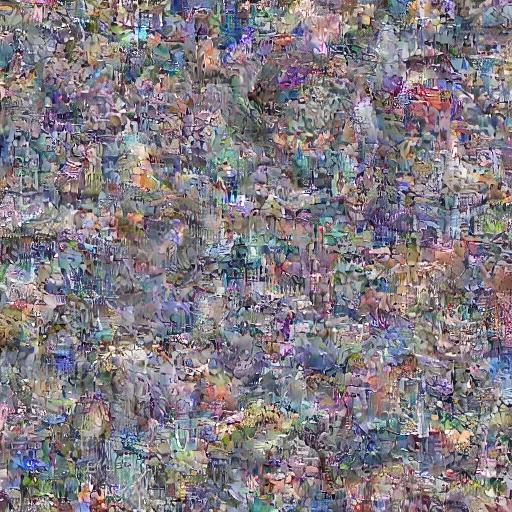
set_random_seed()cfg_512 = HallucinationConfig(prompt="a castle in the clouds", latent_size=128, cutn=128, n_iters=600)final_512, snapshots_512, similarity_512 = hallucinate(cfg_512, vqgan, clip_model, device)print(f"Final similarity at 512x512: {similarity_512:.4f}")save_webp(snapshots_512[0], "direct-512-noise.webp")save_webp(final_512.permute(1, 2, 0).cpu().numpy(), "direct-512-final.webp")
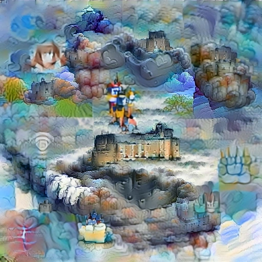
Similarity lands at 0.5407, well above the flagship run’s 0.5038, but the image doesn’t look better for it. The canvas breaks into rectangular patches with visible seams, several of them holding their own separate castle scene, the same kind of artifact called out in “Where the Branch Went After VQGAN+CLIP” above. CLIP still rewards it, since each patch reads as a good match at the crop level even though the whole image doesn’t hold together. Two things plausibly contribute, and one run doesn’t separate them: the decoder is being pushed well past the 256x256 resolution it was trained to reconstruct at, and cutn only doubled while the canvas area quadrupled, so each crop covers proportionally less of the image and neighboring crops overlap less. Dead end either way; the flagship demo stays at 256x256, upscaled afterward with Lanczos instead.
Why Spherical Distance Instead of Cosine Similarity
The loss above is Katherine Crowson’s spherical distance, \(\theta^2/2\) where \(\theta\) is the angle between an image embedding and the text embedding. It’s the same objective the reference notebooks use, and not the more obvious choice. The simpler option is negative mean cosine similarity, \(-\cos(\theta)\), which is what CLIP already outputs directly and what a first pass at this post used too, before testing it against spherical distance. A third natural candidate is plain MSE (mean squared error) between the two embedding vectors, \(\|u-v\|^2\).
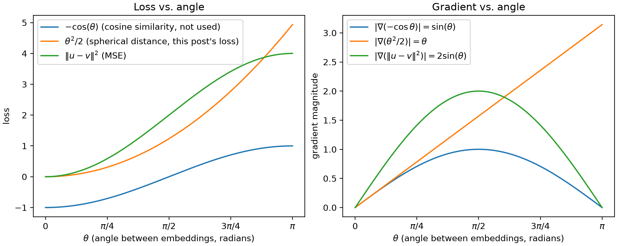
Plotting all three against \(\theta\) shows why cosine similarity and MSE behave identically, and where spherical distance actually differs:
theta = np.linspace(0, np.pi, 200)cosine_loss =-np.cos(theta)spherical_loss = theta**2/2mse_loss =2* (1- np.cos(theta)) # = ||u - v||^2 for unit vectors u, vtheta_ticks = np.array([0, np.pi /4, np.pi /2, 3* np.pi /4, np.pi])theta_tick_labels = ["0", r"$\pi/4$", r"$\pi/2$", r"$3\pi/4$", r"$\pi$"]fig, axes = plt.subplots(1, 2, figsize=(10, 4), constrained_layout=True)axes[0].plot(theta, cosine_loss, label=r"$-\cos(\theta)$(cosine similarity, not used)")axes[0].plot(theta, spherical_loss, label=r"$\theta^2/2$(spherical distance, this post's loss)")axes[0].plot(theta, mse_loss, label=r"$\|u-v\|^2$(MSE)")axes[0].set_xlabel(r"$\theta$(angle between embeddings, radians)")axes[0].set_xticks(theta_ticks, theta_tick_labels)axes[0].set_ylabel("loss")axes[0].set_title("Loss vs. angle")axes[0].legend()axes[1].plot(theta, np.sin(theta), label=r"$|\nabla(-\cos\theta)| = \sin(\theta)$")axes[1].plot(theta, theta, label=r"$|\nabla(\theta^2/2)| = \theta$")axes[1].plot(theta, 2* np.sin(theta), label=r"$|\nabla(\|u-v\|^2)| = 2\sin(\theta)$")axes[1].set_xlabel(r"$\theta$(angle between embeddings, radians)")axes[1].set_xticks(theta_ticks, theta_tick_labels)axes[1].set_ylabel("gradient magnitude")axes[1].set_title("Gradient vs. angle")axes[1].legend()fig.savefig(FIGURES /"loss-gradient-curves.webp", dpi=DPI, pil_kwargs={"lossless": True, "method": 6})plt.close(fig)
Loss and gradient magnitude against the angle between embeddings, for negative cosine similarity, spherical distance and MSE.
The spherical-distance curve is plotted as \(\theta^2/2\) rather than as taming_vqgan_clip.ipynb’s literal \(2\arcsin(\|u-v\|/2)^2\). The two are the same function: for unit vectors separated by \(\theta\), \(\|u-v\| = 2\sin(\theta/2)\), so the arcsin returns exactly \(\theta/2\) and the expression collapses to \(\theta^2/2\).
MSE turns out to be a red herring: for unit vectors, \(\|u-v\|^2 = 2 - 2\cos\theta\), an affine rescaling of \(-\cos\theta\) itself (scale by 2, shift by 2). Its gradient, \(2\sin\theta\), has the exact same shape as cosine similarity’s, just twice the magnitude. Since embeddings here are always L2-normalized before scoring, F.mse_loss would optimize in the same direction as plain cosine similarity, not a different one.
Spherical distance is the one that actually differs. Near \(\theta=0\) it tracks \(-\cos\theta\) closely (both grow roughly as \(\theta^2\)), unsurprisingly, since \(-\cos\theta \approx -1 + \theta^2/2\) for small \(\theta\). The gap opens up in the gradient: \(\sin(\theta)\) peaks at \(\theta=\pi/2\) and fades back toward zero as embeddings approach anti-aligned, while \(\theta\) itself keeps growing. Cosine similarity (and MSE) give a badly-mismatched crop almost no corrective gradient; spherical distance gives it the strongest gradient in the whole range. The cell below turns that shape argument into an actual comparison.
Final similarity, cosine: 0.5065, spherical: 0.5033
Negative cosine similarity
Crowson’s spherical distance
Result, same prompt and seed as the flagship run: 0.5065 with the cosine-similarity loss versus 0.5033 with spherical distance. The two images differ in composition, but neither is sharper or more castle-like than the other.
Cosine similarity comes out ahead here, which is the opposite of what the first run of these same cells produced. Across three executions, with nothing changed but the execution itself, spherical distance led by 0.0014, then trailed by 0.0128, and now trails by 0.0032: the sign flips and the magnitude moves by nearly an order of magnitude. Nondeterminism within a single run points the same way, since the spherical run here and the flagship run above use the same prompt, the same seed and the same configuration and still land 0.0005 apart (0.5033 against 0.5038). The number is a weak instrument besides: hallucinate() returns the mean similarity over cutn random crops taken during the final iteration, measured before that iteration’s optimizer step, so it estimates a slightly stale latent from a random sample of views rather than scoring the image it returns. Combined with cudnn.benchmark=True from the setup cell, there is no reason to trust its fourth decimal place.
So the gradient argument comes out unconfirmed rather than refuted. It predicts a difference in how the two losses treat badly-mismatched crops early in the run, and a single endpoint measurement on one prompt is not the experiment that would expose it: that would need a fixed evaluation crop set, several seeds per loss, and the whole similarity curve rather than its last value. Spherical distance stays HallucinationConfig’s default (see “Scoring and Climbing” above) because it is what every reference implementation uses, which is a weaker reason than I expected to be able to give.
References
Crowson, Katherine, Stella Biderman, Daniel Kornis, et al. 2022. “VQGAN-CLIP: Open Domain Image Generation and Editing with Natural Language Guidance.”arXiv Preprint arXiv:2204.08583.
Esser, Patrick, Robin Rombach, and Björn Ommer. 2021. “Taming Transformers for High-Resolution Image Synthesis.”Proceedings of the IEEE/CVF Conference on Computer Vision and Pattern Recognition (CVPR).
Oppenlaender, Jonas. 2023. “The Cultivated Practices of Text-to-Image Generation.”arXiv Preprint arXiv:2306.11393.
Radford, Alec, Jong Wook Kim, Chris Hallacy, et al. 2021. “Learning Transferable Visual Models from Natural Language Supervision.”arXiv Preprint arXiv:2103.00020.
DeepDream: Google’s 2015 technique that ran gradient ascent on pixels to maximize a frozen CNN’s activations, an early example of the same optimize-the-input idea, aimed at a network’s own activations rather than a CLIP score.↩︎
Big Sleep: an early CLIP-guided image generator built on a pretrained BigGAN, released by the pseudonymous artist advadnoun in early 2021; see lucidrains’ big-sleep implementation.↩︎
VQGAN: Vector-Quantized Generative Adversarial Network; see the official taming-transformers implementation.↩︎
CLIP: Contrastive Language-Image Pre-training, introduced in (Radford et al. 2021).↩︎
Pixray: a modular CLIP-guided image-generation tool built around swappable “drawers.”↩︎