Finally Teaching a Network to See Without Labels

During my PhD in the late 2010s, as a confused student, I read through a lot of blog posts and research papers to follow the new AI trends, although it was not the core of my research. Looking back, I did it for a few reasons: it was far more exciting than my own research area, plain FOMO (fear of missing out), and the time pressure of finishing my PhD while I was struggling to make a breakthrough.

One topic that was particularly interesting to me was self-supervised learning (SSL), and I didn’t fully grasp it at first. At the time, the most intuitive explanation I got was from a Yann LeCun video specifically on self-supervision; he didn’t frame it as energy-based models until later, in a talk that reuses the same slides. I’m linking that later talk here instead, since it also gives a bigger picture, and those familiar slides still start around the 13-minute mark.

One framing from those slides has stuck with me since: self-supervised learning is fundamentally about predicting the missing or transformed part of an input, without a human ever writing down a label. For language, this idea became next-token prediction, now the standard pretraining recipe behind every large language model (LLM). For images, the story took a messier turn: instead of predicting the next patch of pixels, most of the field ended up predicting something under augmentation, i.e., that two differently cropped, jittered, and blurred views of the same photo should land close together in some learned representation space.

I read about this back then, filed it away, forgot about it, revisited it once I had more time, and tried to apply it on wireless spectrum with colleagues (Milosheski et al. 2023). But I never managed to write a post about it. Five years and one long-overdue notebook rewrite later, I finally put it together: I implemented three different self-supervised methods for images from scratch, in plain PyTorch, and trained them on CIFAR-10 to see for myself what makes each one work, and what makes each one break.

This post walks through that experiment, focused on SimCLR: first a short taxonomy of how these methods actually differ mechanically, since “predict something under augmentation” hides a lot of very different engineering, then the SimCLR implementation itself in detail. It turned out to be a genuinely fun way to learn the material, much more hands-on than just reading the papers. I also implemented BYOL and DeepCluster on the same setup, mainly to see how the taxonomy’s other two collapse-avoidance strategies actually play out; both get their own appendices at the end of this post instead of sitting here as equal comparisons.

The Landscape, Formalized

Self-supervised image methods share one recurring problem: the trivial solution to “make two augmented views produce similar outputs” is to map every input to the same constant vector. Two identical vectors are always “similar,” and the training loss is happy. Every method below answers a different question: what stops the network from taking that shortcut?

Contrastive methods (SimCLR (Chen et al. 2020), MoCo (He et al. 2020)) answer with negatives: alongside every pair of views that should look similar, the loss pulls in a batch of other images that should look different and pushes those apart. SimCLR uses the rest of the training batch as negatives; MoCo decouples the count from batch size with a momentum-updated queue instead.

Self-distillation methods (BYOL (Grill et al. 2020), DINO (Caron et al. 2021)) drop negatives entirely: a trained “student” network, a slowly-updated EMA¹ “teacher,” and a small predictor on the student side together supply the asymmetry that stops both networks from drifting to the same constant output. Whether that’s actually enough from scratch on a small dataset is exactly what the BYOL appendix answers the hard way.

Clustering-based methods (DeepCluster (Caron et al. 2018)) sidestep pairwise similarity altogether: periodically cluster the backbone’s features with k-means, then train against those cluster assignments as pseudo-labels. Collapse means every image landing in the same handful of clusters instead of one constant output, fixed by keeping cluster sizes balanced during sampling.

Joint-embedding-predictive methods (I-JEPA (Assran et al. 2023)) reframe the problem itself: predict a masked region’s representation directly from visible context, instead of predicting pixels or matching augmented views, sidestepping collapse through the masking pattern’s own asymmetry.

Method	Family	Prevents collapse via	Implemented here
SimCLR	Contrastive	Negatives (batch)	Yes
MoCo	Contrastive	Negatives (queue)	No
BYOL	Self-distillation	Predictor + EMA asymmetry	Yes (see appendix)
SimSiam	Self-distillation	Stop-gradient alone	No
DINO	Self-distillation	Centering + sharpening	No
DeepCluster	Clustering-based	Balanced cluster sampling	Yes (see appendix)
I-JEPA	Joint-embedding-predictive	Masking asymmetry	No

MoCo and SimSiam (Chen and He 2021) stay conceptual, variations on mechanisms SimCLR and BYOL already cover hands-on. DINO and I-JEPA stay conceptual too, but for a different reason, revisited in “Where the Idea Went.”

The Experiments

All three methods share the same backbone: a ResNet-18 with a CIFAR stem (a 3x3 stride-1 convolution instead of the stock 7x7 stride-2 one, and no initial max-pool), since the ImageNet-tuned stem throws away most of a 32x32 image’s resolution before the first residual block even runs. Everything below is plain PyTorch: hand-written training loops, hand-written losses, no lightning, no lightly. Partly for long-term maintainability (framework APIs drift, hand-written code doesn’t), and partly because showing the actual loss/loop/augmentation code fits a post about understanding these methods better than delegating them to a library.

import gzip
import math
import os
import random
from collections.abc import Iterable
from dataclasses import dataclass
from pathlib import Path
from typing import Any, Final, Optional

import numpy as np
import torch
from matplotlib import pyplot as plt
from torch import Tensor, nn, optim
from torch._inductor import config as inductor_config
from torch.nn import functional as F
from torch.utils import data
from torchvision import datasets, models
from torchvision import transforms as VT

IMAGENET_NORMALIZE = {"mean": (0.485, 0.456, 0.406), "std": (0.229, 0.224, 0.225)}
DATA_ROOT = Path.home() / "datasets" / "cifar10"
SEED: Final[int] = 42
WIDTH: Final[int] = 8  # inches; at dpi=200, renders 2x this blog's ~800px column, no InlineBackend indirection
GOLDEN_RATIO: Final[float] = (1 + math.sqrt(5)) / 2


@dataclass
class Arguments:
    num_workers: int = len(os.sched_getaffinity(0))


args = Arguments()
args

Arguments(num_workers=16)

def set_random_seed(seed: int) -> None:
    random.seed(seed)
    np.random.seed(seed)
    torch.manual_seed(seed)
    torch.cuda.manual_seed(seed)
    torch.cuda.manual_seed_all(seed)


def set_torch_mode(use_optimized: bool, debug: bool) -> None:
    if use_optimized:
        torch.backends.cudnn.benchmark = True
        torch.backends.cudnn.deterministic = False
        torch.backends.cudnn.allow_tf32 = True
        torch.set_float32_matmul_precision("medium")
    else:
        torch.use_deterministic_algorithms(True)
        torch.backends.cudnn.benchmark = False
        torch.backends.cudnn.deterministic = True
        torch.set_float32_matmul_precision("high")
        os.environ["CUBLAS_WORKSPACE_CONFIG"] = ":4096:8"

    # torch.compile is otherwise chatty during autotuning: it prints a full
    # kernel-comparison table for every op it benchmarks.
    inductor_config.trace.log_autotuning_results = False

    if not debug:
        torch.autograd.set_detect_anomaly(False)
        torch.autograd.profiler.profile(False)
        torch.autograd.profiler.emit_nvtx(False)

    print(f"Using {'optimized' if use_optimized else 'deterministic'} mode")
    print(f"Debug functionalities are {'enabled' if debug else 'disabled'}")


set_torch_mode(use_optimized=True, debug=False)
set_random_seed(SEED)

Using optimized mode
Debug functionalities are disabled

def make_cifar_resnet(in_channels: int = 3) -> nn.Module:
    """ResNet-18 with a CIFAR-style stem: 3x3 stride-1 conv, no initial maxpool.

    The stock torchvision resnet18() stem (7x7 stride-2 conv + maxpool) is tuned for
    224x224 ImageNet inputs; on CIFAR-10's 32x32 images it throws away most of the
    spatial resolution before the first residual block even runs.
    """
    resnet = models.resnet18()
    resnet.conv1 = nn.Conv2d(in_channels, 64, kernel_size=3, stride=1, padding=1, bias=False)
    resnet.maxpool = nn.Identity()
    return resnet


class SobelFilter(nn.Module):
    """Fixed grayscale-then-Sobel edge filter (no learned parameters).

    DeepCluster uses this ahead of its backbone so that k-means clusters on shape and
    texture instead of finding the trivial shortcut of clustering by color.
    """

    def __init__(self) -> None:
        super().__init__()
        gray_weight = torch.tensor([0.2989, 0.5870, 0.1140]).view(1, 3, 1, 1)
        kernel_x = torch.tensor([[-1.0, 0.0, 1.0], [-2.0, 0.0, 2.0], [-1.0, 0.0, 1.0]])
        sobel_weight = torch.stack([kernel_x, kernel_x.t()]).unsqueeze(1)
        self.register_buffer("gray_weight", gray_weight)
        self.register_buffer("sobel_weight", sobel_weight)

    def forward(self, x: Tensor) -> Tensor:
        x = F.conv2d(x, self.gray_weight)
        return F.conv2d(x, self.sobel_weight, padding=1)


class ProjectionHead(nn.Module):
    """Linear -> BatchNorm -> ReLU -> Linear -> BatchNorm. Used as SimCLR/BYOL's projector and
    BYOL's predictor. The trailing BatchNorm (no final activation) matches lightly's
    SimCLRProjectionHead, which applies BatchNorm after every linear layer including the last."""

    def __init__(self, in_dim: int = 512, hidden_dim: int = 2048, out_dim: int = 2048) -> None:
        super().__init__()
        self.net = nn.Sequential(
            nn.Linear(in_dim, hidden_dim),
            nn.BatchNorm1d(hidden_dim),
            nn.ReLU(inplace=True),
            nn.Linear(hidden_dim, out_dim),
            nn.BatchNorm1d(out_dim),
        )

    def forward(self, x: Tensor) -> Tensor:
        return self.net(x)


def nt_xent_loss(z0: Tensor, z1: Tensor, temperature: float = 0.5) -> Tensor:
    """SimCLR's NT-Xent / InfoNCE loss between two batches of augmented-view projections."""
    batch_size = z0.shape[0]
    z = F.normalize(torch.cat([z0, z1], dim=0), dim=1)

    similarity = z @ z.t() / temperature
    similarity.fill_diagonal_(-torch.inf)

    positive_idx = torch.arange(batch_size, device=z.device)
    targets = torch.cat([positive_idx + batch_size, positive_idx])
    return F.cross_entropy(similarity, targets)


def byol_loss(p: Tensor, z: Tensor) -> Tensor:
    """BYOL's negative cosine similarity between an online prediction and a stop-gradient target projection."""
    p = F.normalize(p, dim=1)
    z = F.normalize(z, dim=1)
    return 2 - 2 * (p * z).sum(dim=1).mean()


@torch.no_grad()
def update_moving_average(target: nn.Module, online: nn.Module, tau: float) -> None:
    """In-place EMA update of `target`'s parameters and buffers towards `online`, used by BYOL's target network."""
    for target_param, online_param in zip(target.parameters(), online.parameters(), strict=True):
        target_param.mul_(tau).add_(online_param, alpha=1 - tau)
    for target_buffer, online_buffer in zip(target.buffers(), online.buffers(), strict=True):
        target_buffer.copy_(online_buffer)


def byol_tau_schedule(step: int, total_steps: int, tau_base: float) -> float:
    """BYOL paper's cosine ramp: tau starts at `tau_base` and rises to 1.0 by the final step, so
    the target network mixes in less of the online network's per-step change as training
    progresses - a near-frozen target late in training gives the predictor stable regression
    targets, unlike the fixed tau used in earlier attempts (see train_byol's docstring)."""
    progress = min(step / total_steps, 1.0)
    return 1.0 - (1.0 - tau_base) * (math.cos(math.pi * progress) + 1) / 2

def build_augment(strength: str = "full") -> VT.Compose:
    """Augmentation pipeline shared by all three methods, at three preset strengths.

    "full": crop + color jitter + grayscale + blur + flip - SimCLR/BYOL's paired views,
    where augmentation *is* the training signal, not just regularization.
    "light": crop + flip only - DeepCluster's pseudo-label training pass.
    "none": no augmentation - DeepCluster's feature-extraction/clustering pass (clustering
    on noisy augmented features would make cluster assignments unstable run to run) and eval.
    """
    normalize = VT.Normalize(mean=IMAGENET_NORMALIZE["mean"], std=IMAGENET_NORMALIZE["std"])

    if strength == "none":
        return VT.Compose([VT.ToTensor(), normalize])

    transform_steps = [VT.RandomResizedCrop(32, scale=(0.2, 1.0)), VT.RandomHorizontalFlip()]

    if strength == "full":
        transform_steps += [
            VT.RandomApply([VT.ColorJitter(0.4, 0.4, 0.4, 0.1)], p=0.8),
            VT.RandomGrayscale(p=0.2),
            VT.RandomApply([VT.GaussianBlur(kernel_size=3)], p=0.5),
        ]
    elif strength != "light":
        raise ValueError(f"Unknown augmentation strength: {strength!r}")

    transform_steps += [VT.ToTensor(), normalize]
    return VT.Compose(transform_steps)


class TwoViews:
    """Applies a transform twice, producing the (x0, x1) positive pair used by SimCLR/BYOL."""

    def __init__(self, transform: VT.Compose) -> None:
        self.transform = transform

    def __call__(self, x: Any) -> tuple[Tensor, Tensor]:
        return self.transform(x), self.transform(x)


@torch.no_grad()
def extract_embeddings(
    forward_fn: Any, loader: data.DataLoader, device: torch.device
) -> tuple[np.ndarray, np.ndarray]:
    """Runs `forward_fn` (already in eval mode) over a loader, returning (embeddings, labels) as numpy arrays."""
    all_embeddings, all_labels = [], []
    for samples, labels in loader:
        embeddings = forward_fn(samples.to(device)).flatten(start_dim=1)
        all_embeddings.append(embeddings.cpu())
        all_labels.append(labels)
    return torch.cat(all_embeddings).float().numpy(), torch.cat(all_labels).numpy()


def save_checkpoint(
    path: Path,
    model: nn.Module,
    optimizer: optim.Optimizer,
    epoch: int,
    scheduler: Any = None,
    loss_history: list[float] | None = None,
    best_loss: float | None = None,
) -> None:
    """Gzip-compressed checkpoint. Model weights don't compress dramatically (fairly high-entropy
    floats), but it's free - no extra dependency, no precision loss - so there's no reason not to.

    Also saves RNG state (Python/NumPy/torch CPU/torch CUDA) plus loss_history/best_loss, so a
    resumed run continues the same random stream instead of replaying identical batches and
    augmentation choices from a fixed seed - see load_checkpoint's `restore_rng`.
    """
    checkpoint = {
        "model": model.state_dict(),
        "optimizer": optimizer.state_dict(),
        "epoch": epoch,
        "rng_state": {
            "random": random.getstate(),
            "numpy": np.random.get_state(),
            "torch": torch.get_rng_state(),
            "cuda": torch.cuda.get_rng_state_all() if torch.cuda.is_available() else None,
        },
    }
    if scheduler is not None:
        checkpoint["scheduler"] = scheduler.state_dict()
    if loss_history is not None:
        checkpoint["loss_history"] = loss_history
    if best_loss is not None:
        checkpoint["best_loss"] = best_loss
    with gzip.open(path, "wb") as f:
        torch.save(checkpoint, f)


def load_checkpoint(
    path: Path,
    model: nn.Module,
    optimizer: optim.Optimizer = None,
    scheduler: Any = None,
    restore_rng: bool = False,
) -> dict[str, Any]:
    """Auto-detects gzip (via its magic bytes) so this loads both the new compressed checkpoints
    and the plain ones already on disk from before compression was added.

    `restore_rng=True` resets Python/NumPy/torch RNG state to exactly where training left off -
    only meaningful when actually resuming a training loop (not for eval-only loading, where the
    notebook's own fixed-seed `set_random_seed()` call should stay in charge instead). Returns
    the epoch/loss_history/best_loss a resuming train_* function needs; old checkpoints predating
    this - like the first SimCLR run's `epoch_200.pt` - simply lack those keys and default sanely.

    `weights_only=False`: these checkpoints carry RNG state (Python/NumPy tuples, not just
    tensors), which PyTorch's default `weights_only=True` refuses to unpickle. Safe here since
    every checkpoint this loads is one this notebook produced itself, not a third-party file.
    """
    with open(path, "rb") as f:
        is_gzip = f.read(2) == b"\x1f\x8b"
    opener = gzip.open if is_gzip else open
    with opener(path, "rb") as f:
        checkpoint = torch.load(f, map_location="cpu", weights_only=False)
    model.load_state_dict(checkpoint["model"])
    if optimizer is not None and "optimizer" in checkpoint:
        optimizer.load_state_dict(checkpoint["optimizer"])
    if scheduler is not None and "scheduler" in checkpoint:
        scheduler.load_state_dict(checkpoint["scheduler"])
    if restore_rng and "rng_state" in checkpoint:
        rng = checkpoint["rng_state"]
        random.setstate(rng["random"])
        np.random.set_state(rng["numpy"])
        torch.set_rng_state(rng["torch"])
        if rng["cuda"] is not None and torch.cuda.is_available():
            torch.cuda.set_rng_state_all(rng["cuda"])
    return {
        "epoch": checkpoint["epoch"],
        "loss_history": checkpoint.get("loss_history", []),
        "best_loss": checkpoint.get("best_loss", float("inf")),
    }


def load_resume_state(
    resume_from: Path | None,
    model: nn.Module,
    optimizer: optim.Optimizer = None,
    scheduler: Any = None,
) -> tuple[int, list[float], float]:
    """Shared resume-state loading for all three train_* functions - they only differ in which
    of optimizer/scheduler they pass through (DeepCluster passes neither, since it rebuilds both
    fresh every reclustering round regardless of resume). Returns (start_epoch, loss_history,
    best_loss), at fresh-start defaults (0, [], inf) if `resume_from` is None.
    """
    if resume_from is None:
        return 0, [], float("inf")
    resumed = load_checkpoint(resume_from, model, optimizer, scheduler, restore_rng=True)
    return resumed["epoch"], resumed["loss_history"], resumed["best_loss"]

class UnNormalize:
    def __init__(self, mean: Iterable[float], std: Iterable[float]):
        self.mean = mean
        self.std = std

    def __call__(self, tensor: Tensor) -> Tensor:
        for t, m, s in zip(tensor, self.mean, self.std, strict=True):
            t.mul_(s).add_(m)
        return tensor


reverse_transform = VT.Compose(
    [
        UnNormalize(mean=IMAGENET_NORMALIZE["mean"], std=IMAGENET_NORMALIZE["std"]),
        VT.ToPILImage(),
    ]
)

device = torch.device("cuda" if torch.cuda.is_available() else "cpu")

### Self-supervised pretraining dataset: SimCLR/BYOL need two full-strength augmented views per image
pretrain_transform = TwoViews(build_augment("full"))
pretrainset = datasets.CIFAR10(root=DATA_ROOT, train=True, download=False, transform=pretrain_transform)
pretrain_loader = data.DataLoader(
    pretrainset, batch_size=256, shuffle=True, drop_last=True, pin_memory=True, num_workers=args.num_workers
)

### Classification training (linear probe) and evaluation: no augmentation
eval_transform = build_augment("none")
trainset = datasets.CIFAR10(root=DATA_ROOT, train=True, download=False, transform=eval_transform)
trainset_loader = data.DataLoader(
    trainset, batch_size=256, shuffle=True, drop_last=True, pin_memory=True, num_workers=args.num_workers
)

testset = datasets.CIFAR10(root=DATA_ROOT, train=False, download=False, transform=eval_transform)
testset_loader = data.DataLoader(testset, batch_size=256, shuffle=False, drop_last=False, num_workers=args.num_workers)

### Visualization testset (raw PIL images, for the image-mapped t-SNE plot)
vis_testset = datasets.CIFAR10(root=DATA_ROOT, train=False, download=False, transform=None)

/home/gcerar/workspace/gcerar.github.io/.venv/lib/python3.12/site-packages/torchvision/datasets/cifar.py:83: VisibleDeprecationWarning: dtype(): align should be passed as Python or NumPy boolean but got `align=0`. Did you mean to pass a tuple to create a subarray type? (Deprecated NumPy 2.4)
  entry = pickle.load(f, encoding="latin1")

SimCLR

SimCLR is the simplest of the three to state formally, since its collapse-prevention mechanism is also its whole loss function. Given a batch of \(N\) images, two augmented views \(x_i\), \(x_i'\) are drawn per image, giving \(2N\) views total. Each passes through the backbone and a small projection head to produce embeddings \(z_i\), \(z_i'\). The NT-Xent² loss then treats \(z_i\) and \(z_i'\) as a positive pair, and every other view in the batch as a negative:

\[ \mathcal{L}_i = -\log \frac{\exp(\mathrm{sim}(z_i, z_i') / \tau)}{\exp(\mathrm{sim}(z_i, z_i') / \tau) + \sum_{j \neq i} \left[\exp(\mathrm{sim}(z_i, z_j) / \tau) + \exp(\mathrm{sim}(z_i, z_j') / \tau)\right]} \]

where \(\mathrm{sim}(\cdot,\cdot)\) is cosine similarity, \(\tau\) is a temperature (0.5 here), and \(j\) ranges over every image other than \(i\) in the batch, so the denominator sums over all \(2N - 1\) other views: the positive pair itself plus both views of every other image. This is exactly the “push positives together, negatives apart” mechanism from the taxonomy above, and it’s the reason SimCLR doesn’t need anything cleverer to avoid collapse: a constant embedding makes every negative pair equally “similar” to every positive pair, so the denominator swamps the numerator and the loss stays high.

Note

A worked example. Take a tiny batch of \(N=2\) images (\(2N=4\) views total) and temperature \(\tau=0.5\). Say the backbone gives cosine similarities \(\mathrm{sim}(z_1, z_1') = 0.8\) for the positive pair, and \(\mathrm{sim}(z_1, z_2) = 0.1\), \(\mathrm{sim}(z_1, z_2') = 0.05\) for the two views of the one other image (the negatives). Plugging into the formula for \(\mathcal{L}_1\):

\[ \mathcal{L}_1 = -\log \frac{\exp(0.8 / 0.5)}{\exp(0.8 / 0.5) + \exp(0.1 / 0.5) + \exp(0.05 / 0.5)} = -\log \frac{4.95}{4.95 + 1.22 + 1.11} \approx -\log(0.68) \approx 0.39 \]

Now compare the collapsed case: if the backbone mapped every image to the same vector, every similarity above would be \(1.0\) instead, and the loss becomes \(-\log(1/3) \approx 1.10\), nearly three times higher. That’s the whole mechanism in one number: collapsing doesn’t cheat the loss; it makes it worse, since a constant embedding can’t tell the positive apart from the negatives either.

A batch of augmented images, one contrastive loss, and the negatives inside the same batch do all the work of preventing collapse.

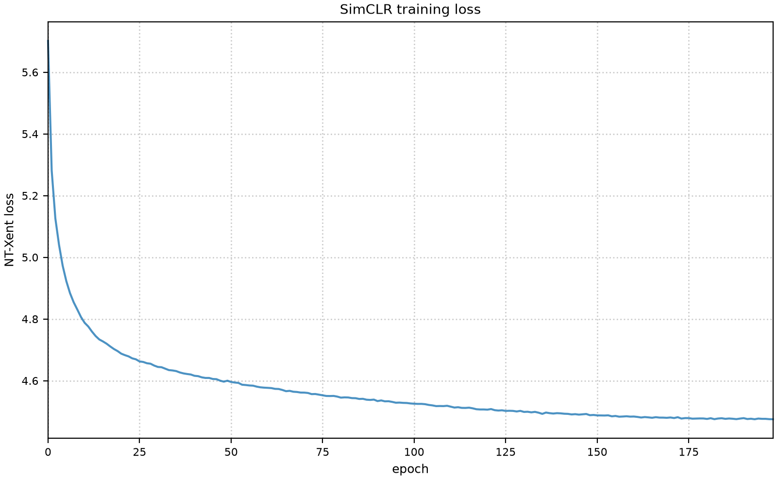
The augmentation pipeline (random resized crop, color jitter, grayscale, Gaussian blur, horizontal flip) is the training signal here, not regularization: the backbone can only learn to ignore what augmentation varies, so weak augmentation means a weak, easily satisfied task. I trained SimCLR twice. The first attempt used a flat learning rate with a ReduceLROnPlateau scheduler that never actually triggered (its threshold was looser than the loss’s real epoch-to-epoch noise), and plateaued around 4.49 after roughly 150 epochs, still under-converged. The second used a proper warmup-then-cosine-decay schedule instead, ran 200 epochs (~14s/epoch on an RTX 3090), and converged cleanly to a final loss of 4.475 as the learning rate decayed to zero. Only a modest improvement over the first run’s plateau, which is itself informative: ~4.47-4.49 looks like this setup’s actual floor for this backbone, batch size, and temperature.

from tqdm.auto import tqdm


class SimCLRModel(nn.Module):
    """Backbone + projection head. The projected output feeds the NT-Xent loss; the backbone
    output (before the projector) is what every evaluation and visualization cell uses."""

    def __init__(self) -> None:
        super().__init__()
        resnet = make_cifar_resnet()
        self.backbone = nn.Sequential(*list(resnet.children())[:-1])
        self.projector = ProjectionHead(512, 2048, 2048)

    def forward(self, x: Tensor) -> Tensor:
        return self.projector(self.backbone(x).flatten(start_dim=1))


def train_simclr(
    model: SimCLRModel,
    loader: data.DataLoader,
    epochs: int,
    device: torch.device,
    checkpoint_path: Path = Path("./checkpoints/simclr/best.pt.gz"),
    warmup_epochs: int = 10,
    resume_from: Path | None = None,
) -> list[float]:
    """Saves (overwriting) whenever the epoch loss improves on the best seen so far - NT-Xent's
    negatives make a lower loss a reliable "better" signal here, unlike BYOL's loss (see train_byol).
    Also unconditionally saves the true final-epoch state to "final.pt.gz" once training completes,
    for comparison against "best.pt.gz" (see train_byol's docstring for why that comparison matters).

    `resume_from`, if given, restores model/optimizer/scheduler/RNG state and continues from the
    saved epoch, rather than restarting the shuffle order, augmentation randomness, and LR
    schedule from scratch.
    """
    model.to(device)
    model = torch.compile(model)
    optimizer = optim.Adam(model.parameters(), lr=1e-3, fused=device.type == "cuda")
    # ReduceLROnPlateau never triggered in practice (its eps=0.5 threshold was looser than the
    # loss's actual epoch-to-epoch noise) - a real warmup + cosine decay replaces it here, same
    # as train_byol.
    warmup = optim.lr_scheduler.LinearLR(optimizer, start_factor=0.01, total_iters=warmup_epochs)
    cosine = optim.lr_scheduler.CosineAnnealingLR(optimizer, T_max=epochs - warmup_epochs)
    scheduler = optim.lr_scheduler.SequentialLR(optimizer, schedulers=[warmup, cosine], milestones=[warmup_epochs])
    checkpoint_path.parent.mkdir(parents=True, exist_ok=True)

    start_epoch, loss_history, best_loss = load_resume_state(resume_from, model, optimizer, scheduler)

    for epoch in tqdm(range(start_epoch, epochs), desc="SimCLR", initial=start_epoch, total=epochs):
        model.train()
        epoch_loss = 0.0
        for (x0, x1), _ in loader:
            x0, x1 = x0.to(device), x1.to(device)
            with torch.autocast(device_type=device.type, dtype=torch.bfloat16):
                loss = nt_xent_loss(model(x0), model(x1))

            optimizer.zero_grad()
            loss.backward()
            optimizer.step()
            epoch_loss += loss.item()

        epoch_loss /= len(loader)
        loss_history.append(epoch_loss)
        scheduler.step()

        if epoch_loss < best_loss:
            best_loss = epoch_loss
            save_checkpoint(checkpoint_path, model, optimizer, epoch + 1, scheduler, loss_history, best_loss)

    save_checkpoint(
        checkpoint_path.parent / "final.pt.gz", model, optimizer, epochs, scheduler, loss_history, best_loss
    )
    return loss_history


simclr_model = SimCLRModel()

# First attempt (ReduceLROnPlateau) plateaued under-converged (see prose above); retrained with
# the warmup+cosine schedule above instead. NT-Xent's negatives prevent the collapse BYOL hit,
# so best.pt.gz is trustworthy directly, no separate diagnostic needed.
# simclr_loss_history = train_simclr(simclr_model, pretrain_loader, epochs=200, device=device)

simclr_checkpoint = load_checkpoint(Path("./checkpoints/simclr/best.pt.gz"), simclr_model)

fig, ax = plt.subplots(figsize=(WIDTH, WIDTH / GOLDEN_RATIO), dpi=200, constrained_layout=True)
ax.plot(
    range(len(simclr_checkpoint["loss_history"])),
    simclr_checkpoint["loss_history"],
    linewidth=1.5,
    alpha=0.80,
    clip_on=False,
)
ax.set_xlabel("epoch", fontsize=9)
ax.set_ylabel("NT-Xent loss", fontsize=9)
ax.set_title("SimCLR training loss", fontsize=10)
ax.tick_params(labelsize=8)
ax.autoscale(axis="x", tight=True)  # epoch 0 starts flush against the y-axis, no left margin
ax.grid(color="0.8", linestyle=":", linewidth=1)
plt.show()

I also trained BYOL and DeepCluster on the same backbone and CIFAR-10 setup; both get their own write-ups in the appendices below rather than a full walkthrough here.

Evaluating the Representations

Two evaluations for SimCLR: a linear probe (freeze the backbone, train a single linear layer on top, the standard protocol in this literature) and k-NN classification on the frozen embeddings directly (no training at all, cheap, and DINO’s convention for a training-free sanity check). BYOL’s and DeepCluster’s numbers exist too, just not here: see their appendices, where each is the point of its own section rather than a footnote to this one.

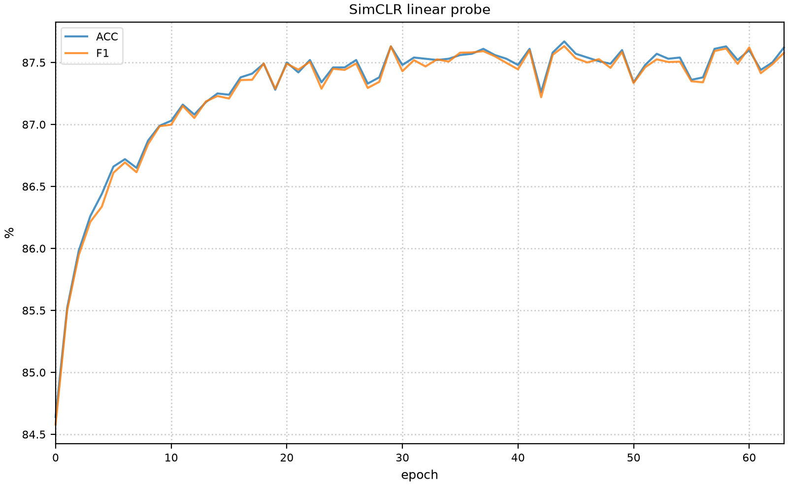
One methodology fix versus the original version of this notebook: the linear probe here trains on one split and evaluates on a held-out one. The original notebook’s classifier trained and validated on the same test set, so its reported 80.9% accuracy was itself partly a training-set number. The result below isn’t directly comparable to that old baseline for this reason, on top of everything else that changed (framework, backbone, training length).

from sklearn.metrics import accuracy_score, f1_score


class LinearProbeModel(nn.Module):
    """Combines a frozen backbone with a linear_probe's trained classifier head into one
    callable module - used by the attribution-map cells, which need a single forward pass
    from image to class logits."""

    def __init__(self, backbone: nn.Module, classifier: nn.Module) -> None:
        super().__init__()
        self.backbone = backbone
        self.classifier = classifier

    def forward(self, x: Tensor) -> Tensor:
        return self.classifier(self.backbone(x).flatten(start_dim=1))


def linear_probe(
    backbone: nn.Module,
    train_loader: data.DataLoader,
    test_loader: data.DataLoader,
    epochs: int,
    device: torch.device,
    label: str = "",
) -> dict[str, Any]:
    """Freezes `backbone` and trains a single linear layer on top of it, plotting ACC/F1 per epoch."""
    backbone = backbone.to(device).eval()
    backbone = torch.compile(backbone)
    for param in backbone.parameters():
        param.requires_grad = False

    classifier = nn.Linear(512, 10).to(device)
    optimizer = optim.Adam(classifier.parameters(), lr=1e-3, fused=device.type == "cuda")
    scheduler = optim.lr_scheduler.ReduceLROnPlateau(optimizer, eps=0.5)

    acc = f1 = 0.0
    acc_history: list[float] = []
    f1_history: list[float] = []
    for _epoch in tqdm(range(epochs), desc="linear probe"):
        classifier.train()
        for inputs, targets in train_loader:
            inputs, targets = inputs.to(device), targets.to(device)
            with torch.no_grad():
                features = backbone(inputs).flatten(start_dim=1)
            loss = F.cross_entropy(classifier(features), targets)

            optimizer.zero_grad()
            loss.backward()
            optimizer.step()

        classifier.eval()
        labels_true, labels_pred = [], []
        with torch.no_grad():
            for inputs, targets in test_loader:
                features = backbone(inputs.to(device)).flatten(start_dim=1)
                labels_true.append(targets)
                labels_pred.append(torch.argmax(classifier(features), dim=1).cpu())

        y_true = torch.cat(labels_true).numpy()
        y_pred = torch.cat(labels_pred).numpy()
        acc = accuracy_score(y_true, y_pred)
        f1 = f1_score(y_true, y_pred, average="weighted")
        acc_history.append(acc)
        f1_history.append(f1)
        scheduler.step(acc)

    epochs_range = range(epochs)
    fig, ax = plt.subplots(figsize=(WIDTH, WIDTH / GOLDEN_RATIO), dpi=200, constrained_layout=True)
    ax.plot(epochs_range, [a * 100 for a in acc_history], label="ACC", linewidth=1.5, alpha=0.80, clip_on=False)
    ax.plot(epochs_range, [f * 100 for f in f1_history], label="F1", linewidth=1.5, alpha=0.80, clip_on=False)
    ax.set_xlabel("epoch", fontsize=9)
    ax.set_ylabel("%", fontsize=9)
    ax.set_title(f"{label} linear probe" if label else "linear probe", fontsize=10)
    ax.tick_params(labelsize=8)
    ax.autoscale(axis="x", tight=True)  # epoch 0 starts flush against the y-axis, no left margin
    ax.legend(prop={"size": 8}, framealpha=0.6)
    ax.grid(color="0.8", linestyle=":", linewidth=1)
    plt.show()

    return {"accuracy": acc, "f1": f1, "classifier": classifier, "model": LinearProbeModel(backbone, classifier)}

from sklearn.neighbors import KNeighborsClassifier


def knn_evaluate(
    train_embeddings: np.ndarray,
    train_labels: np.ndarray,
    test_embeddings: np.ndarray,
    test_labels: np.ndarray,
    k: int = 20,
) -> float:
    """k-NN accuracy on frozen embeddings - DINO's convention for a training-free evaluation."""
    knn = KNeighborsClassifier(n_neighbors=k, metric="cosine", n_jobs=-1)
    knn.fit(train_embeddings, train_labels)
    return accuracy_score(test_labels, knn.predict(test_embeddings))

from sklearn.model_selection import train_test_split


def data_efficiency_probe(
    backbone: nn.Module,
    train_dataset: datasets.CIFAR10,
    test_loader: data.DataLoader,
    device: torch.device,
    fractions: tuple[float, ...] = (0.01, 0.1, 1.0),
    epochs: int = 20,
) -> dict[float, float]:
    """Linear probe accuracy trained on a stratified fraction of the labeled train set, per fraction.

    This is the actual "fewer labels needed" argument for SSL: if a good representation was
    learned without labels, a linear probe on top of it should need far fewer labeled examples
    to reach a given accuracy than training from scratch would.
    """
    targets = np.array(train_dataset.targets)
    results = {}

    for fraction in fractions:
        if fraction >= 1.0:
            subset = train_dataset
        else:
            indices, _ = train_test_split(
                np.arange(len(train_dataset)), train_size=fraction, stratify=targets, random_state=0
            )
            subset = data.Subset(train_dataset, indices)

        subset_loader = data.DataLoader(subset, batch_size=256, shuffle=True, num_workers=args.num_workers)
        metrics = linear_probe(backbone, subset_loader, test_loader, epochs=epochs, device=device)
        results[fraction] = metrics["accuracy"]
        print(f"fraction {fraction:.0%}: ACC {metrics['accuracy'] * 100:.1f}%")

    return results

Linear probe and k-NN for SimCLR:

### SimCLR - linear probe ACC 87.4% / F1 87.4%, k-NN ACC 86.0%
simclr_backbone = simclr_model.backbone
simclr_linear = linear_probe(
    simclr_backbone, trainset_loader, testset_loader, epochs=64, device=device, label="SimCLR"
)
simclr_train_emb, simclr_train_labels = extract_embeddings(simclr_backbone.eval(), trainset_loader, device)
simclr_test_emb, simclr_test_labels = extract_embeddings(simclr_backbone.eval(), testset_loader, device)
simclr_knn = knn_evaluate(simclr_train_emb, simclr_train_labels, simclr_test_emb, simclr_test_labels)
# simclr_data_efficiency = data_efficiency_probe(simclr_backbone, trainset, testset_loader, device=device)

87.4% linear-probe accuracy and 86.0% k-NN accuracy are solid numbers for a from-scratch, 200-epoch CIFAR-10 run with no labels involved in pretraining. That’s consistent with the mechanism itself: negatives are a strong, direct collapse-prevention signal, and a contrastive objective trained end-to-end pushes the backbone directly toward separable features, exactly what a linear probe rewards. For a direct look at the embeddings themselves, rather than just these numbers, here they are.

Does It Look Like It Learned Something?

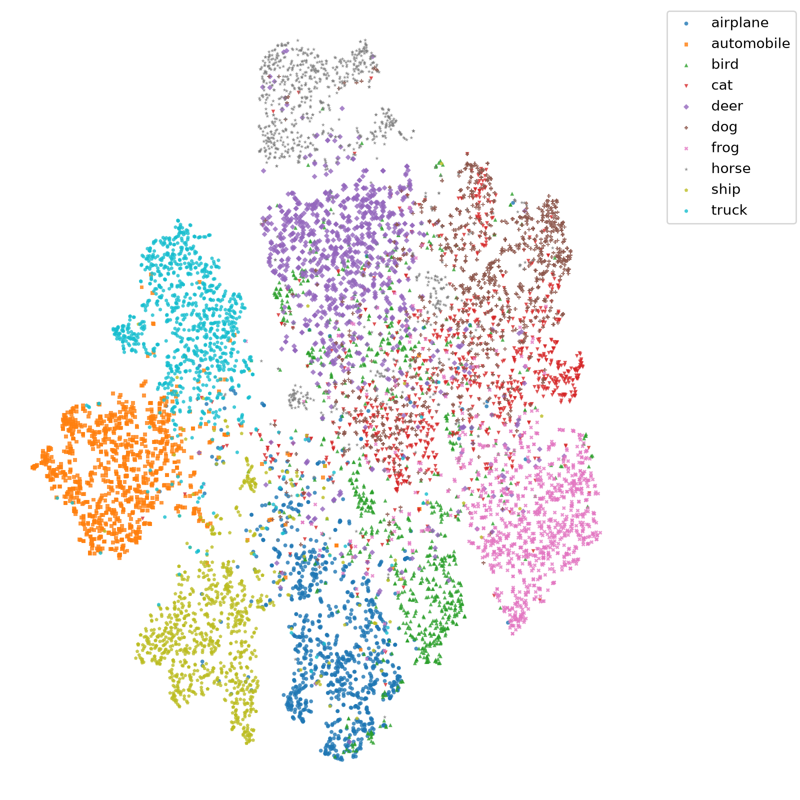
Two broad regions emerge without the model ever seeing a label: manufactured vehicles (cars, trucks, ships, planes) cluster on the left, living things (horses, deer, dogs, cats, birds, frogs) on the right. Each side has its own finer structure too: cars and trucks separate from boats and ships, four-legged mammals separate from birds, frogs, and other small animals. None of this structure was ever labeled during pretraining; it comes entirely from which augmented views of which images the backbone learned to treat as similar. SimCLR clearly learned something real here. Its contrastive mechanism has practical costs of its own, though, which is exactly where the rest of the field went next.

### Image-mapped t-SNE embeddings for SimCLR - actual CIFAR-10 thumbnails placed at their
### frozen test-set t-SNE coordinates, instead of plain dots. Self-contained (duplicates the
### DeepCluster appendix's tsne_pipeline/plot_embeddings setup below) rather than reordering
### cells, so this cell only depends on cell 10's already-loaded simclr_model checkpoint, not
### the appendix.
from matplotlib import offsetbox
from PIL.Image import Image as PILImage
from sklearn.manifold import TSNE
from sklearn.pipeline import Pipeline
from sklearn.preprocessing import StandardScaler

tsne_pipeline = Pipeline([("scaler", StandardScaler()), ("tsne", TSNE(n_jobs=-1, random_state=42))])

vis_samples = np.asarray([x for x, _ in vis_testset])


def plot_embeddings(
    x1: np.ndarray,
    x2: np.ndarray,
    samples: Iterable[np.ndarray | PILImage | Tensor],
    min_distance: float = 0.1,
    zoom: float = 0.5,
    ax: Any | None = None,
) -> Any:
    if ax is None:
        ax = plt.gca()

    X = np.stack([x1, x2], axis=-1)
    shown_images = np.array([[np.inf, np.inf]])
    for i in range(X.shape[0]):
        dist = np.sum((X[i] - shown_images) ** 2, 1)
        if np.min(dist) < min_distance:
            continue

        sample = samples[i]
        if isinstance(sample, Tensor):
            sample = sample.permute(1, 2, 0).numpy()
        if isinstance(sample, PILImage):
            sample = np.asarray(sample)

        shown_images = np.r_[shown_images, [X[i]]]
        im = offsetbox.OffsetImage(sample, zoom=zoom)
        ab = offsetbox.AnnotationBbox(offsetbox=im, xy=X[i], frameon=False)
        ax.add_artist(ab)

    return ax


simclr_backbone_gpu = simclr_model.backbone.to(device).eval()
simclr_embeddings, _ = extract_embeddings(simclr_backbone_gpu, testset_loader, device)
simclr_projection = tsne_pipeline.fit_transform(simclr_embeddings)

fig, ax = plt.subplots(figsize=(WIDTH, WIDTH), dpi=200)
ax.axis("off")
ax.scatter(simclr_projection[:, 0], simclr_projection[:, 1], marker=".", edgecolors="none", alpha=0.0)
plot_embeddings(simclr_projection[:, 0], simclr_projection[:, 1], samples=vis_samples, ax=ax)
plt.tight_layout()
plt.show()

/tmp/ipykernel_2248013/825782251.py:57: UserWarning: Tight layout not applied. The left and right margins cannot be made large enough to accommodate all Axes decorations.
  plt.tight_layout()

The same projection, colored by true label instead of shown as thumbnails, makes the cluster boundaries easier to read at a glance:

### Class-colored t-SNE embeddings for SimCLR - same projection as the image-mapped version
### above, colored by true label instead of shown as thumbnails.
import matplotlib as mpl

classes = ["airplane", "automobile", "bird", "cat", "deer", "dog", "frog", "horse", "ship", "truck"]
cmap = mpl.colormaps.get_cmap("tab10")
vis_labels = np.asarray([label for _, label in vis_testset])

fig, ax = plt.subplots(figsize=(WIDTH, WIDTH), dpi=200)
for class_idx in sorted(set(vis_labels)):
    ax.scatter(
        simclr_projection[vis_labels == class_idx, 0],
        simclr_projection[vis_labels == class_idx, 1],
        color=cmap(class_idx),
        marker=".",
        edgecolors="none",
        alpha=0.8,
        label=classes[class_idx],
    )
ax.axis("off")
ax.legend(bbox_to_anchor=(1.05, 1), loc="upper left")
plt.tight_layout()
plt.show()

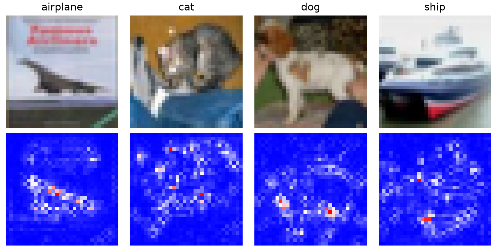
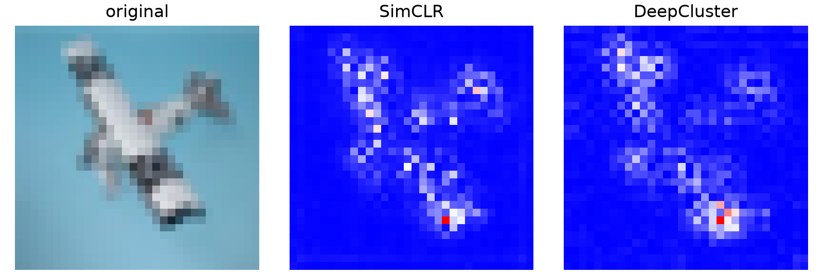
A few GuidedBackprop examples show what the linear-probe classifier keys on for its predictions:

### GuidedBackprop attribution for SimCLR, a few examples spanning different classes.
from copy import deepcopy

from captum.attr import GuidedBackprop

example_classes = [0, 3, 5, 8]  # airplane, cat, dog, ship - two from each supercluster above
targets_array = np.asarray(testset.targets)
example_indices = [int(np.flatnonzero(targets_array == label)[0]) for label in example_classes]

simclr_probe_model = deepcopy(simclr_linear["model"]).eval()
gbp = GuidedBackprop(simclr_probe_model)

fig, axes = plt.subplots(nrows=2, ncols=len(example_indices), figsize=(WIDTH, WIDTH / 2), dpi=200)
for col, idx in enumerate(example_indices):
    sample_norm, sample_label = testset[idx]
    sample_image = reverse_transform(sample_norm.clone())

    attr = gbp.attribute(sample_norm.unsqueeze(0).to(device), target=sample_label)
    attr = attr.squeeze().permute(1, 2, 0).cpu().numpy()
    attr = np.sum(np.abs(attr), axis=-1)

    axes[0, col].imshow(sample_image, interpolation="none")
    axes[0, col].set_title(classes[sample_label])
    axes[0, col].axis("off")

    axes[1, col].imshow(attr, cmap="bwr", interpolation="none")
    axes[1, col].axis("off")

plt.tight_layout()
plt.show()

/home/gcerar/workspace/gcerar.github.io/.venv/lib/python3.12/site-packages/captum/attr/_core/guided_backprop_deconvnet.py:63: UserWarning: Input Tensor 0 did not already require gradients, required_grads has been set automatically.
  gradient_mask = apply_gradient_requirements(inputs_tuple)
/home/gcerar/workspace/gcerar.github.io/.venv/lib/python3.12/site-packages/captum/attr/_core/guided_backprop_deconvnet.py:66: UserWarning: Setting backward hooks on ReLU activations.The hooks will be removed after the attribution is finished
  warnings.warn(
/home/gcerar/workspace/gcerar.github.io/.venv/lib/python3.12/site-packages/captum/attr/_core/guided_backprop_deconvnet.py:63: UserWarning: Input Tensor 0 did not already require gradients, required_grads has been set automatically.
  gradient_mask = apply_gradient_requirements(inputs_tuple)
/home/gcerar/workspace/gcerar.github.io/.venv/lib/python3.12/site-packages/captum/attr/_core/guided_backprop_deconvnet.py:66: UserWarning: Setting backward hooks on ReLU activations.The hooks will be removed after the attribution is finished
  warnings.warn(

Where the Idea Went

Contrastive learning’s biggest practical limitation is the one SimCLR’s own design makes obvious: negatives need to come from somewhere, and getting enough of them, reliably, means either very large batches (SimCLR’s own approach, expensive) or a maintained queue of past embeddings (MoCo’s fix). Neither is free. This is part of why the self-distillation family exists at all: BYOL’s whole pitch is that you can drop negatives entirely, at the cost of exactly the collapse risk this post spent an entire appendix on.

DINO pushes the self-distillation idea further than BYOL, and does so with machinery purpose-built for the collapse problem: instead of BYOL’s predictor asymmetry alone, DINO centers and sharpens the teacher’s output distribution, which prevents the specific kind of directional collapse this post’s BYOL attempts kept running into. DeepCluster’s pseudo-labeling has a lineage here too, worth naming since it’s not always obvious from the outside: Caron et al., who wrote the original DeepCluster paper, went on to write SwAV (Caron et al. 2020) and then DINO. SwAV is an online clustering method that swaps DeepCluster’s offline k-means step for a differentiable, batch-level assignment. Three methods, one continuous line of thinking about how to get useful representations out of clustering-flavored self-supervision without ever running an actual k-means step during training. That line kept going past this post’s own timeline too: DINOv2 (Oquab et al. 2023) adds a patch-level self-distillation objective on top of DINO’s image-level one and trains on a curated, web-scale dataset, producing general-purpose visual features strong enough to use frozen, with no fine-tuning, across a wide range of downstream tasks.

I-JEPA reframes the prediction target itself, rather than tweaking how collapse is prevented. Instead of asking two augmented views to match, or asking cluster assignments to be predictable, it masks out a region of an image and predicts that region’s representation, not its pixels, conditioned on the visible context. This sidesteps a subtler problem that pixel-level masked-image-modeling approaches run into: predicting exact pixel values forces the network to spend capacity on details (textures, noise) that may not matter for a downstream task, whereas predicting in representation space lets the network decide what’s worth representing.

None of DINO, DINOv2, SwAV, or I-JEPA get implemented in this post: their collapse-avoidance machinery is tuned for ImageNet-scale data, and a from-scratch CIFAR-10 attempt would likely be too unreliable to trust as evidence either way.

Conclusion

SimCLR learned something real from CIFAR-10 without ever seeing a label, cleanly and reproducibly, which is the main result this post set out to show. I also trained BYOL and DeepCluster on the same setup; both get full write-ups in the appendices below, including a BYOL investigation that never stopped collapsing no matter what I tried, which is worth a look if you only have five minutes.

The idea underneath all of it, predicting a missing or transformed view of your own input without a human ever writing down a label, is the same idea underneath modern language model pretraining, even though the concrete mechanisms (contrastive losses, momentum encoders, k-means pseudo-labels) look nothing like next-token prediction on the surface. That’s the framing I started this post with, from a LeCun course years ago, and it’s held up. The hard part was never the framing: it was always in the details of what stops the trivial solution from winning. That’s exactly what four failed BYOL runs ended up teaching me the hard way.

This CIFAR-10 exercise was also where I first got properly hands-on with DeepCluster, before it became the reference architecture for a later paper on clustering wireless spectrum activity that I worked on with Ljupcho Milosheski (I won’t go into that work here; it’s a separate story). The notebook itself then sat half-finished for five years. Finishing it finally happened with an AI assistant doing a lot of the actual writing alongside me, a fitting way to close a loop that started with a PhD-era course on self-supervised learning.

Appendix

DeepCluster

NoteShow the DeepCluster write-up

DeepCluster’s collapse-prevention problem looks nothing like SimCLR’s or BYOL’s: there’s no pairwise similarity in its loss at all. Training alternates instead: cluster the backbone’s features with k-means into \(k\) pseudo-labels, then train the backbone (plus a fresh linear head) to predict them with ordinary cross-entropy, exactly as if they were real classes. Repeat.

The clusters are the labels. There’s no “similar to what” question here, only “similar to which of these \(k\) made-up categories.”

Collapse takes a different shape here: instead of one constant embedding, every image lands in the same handful of clusters, degenerating the pseudo-label task into predicting a near-constant output anyway. Two mitigations from the original paper (Caron et al. 2018) address this: inverse-frequency sampling so no cluster dominates the gradient (WeightedRandomSampler), and Sobel-filtering the input so clustering keys on shape and texture instead of the trivial shortcut of color.

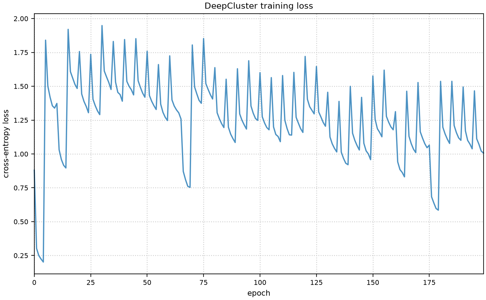
I trained two versions. The first reclustered every epoch, matching the original paper’s cadence: 200 epochs, all 100 clusters stayed populated, NMI³ against the true CIFAR-10 labels came out to 0.18, a modest but genuine signal. The second reclustered only every 5 epochs, a cadence I found in another DeepCluster-based codebase rather than the paper itself, and it won on both fronts: faster (4 of 5 epochs skip the expensive feature-extraction-and-k-means step) and better (NMI 0.189, a loss that kept dropping instead of plateauing). Reclustering less often gives the backbone more consecutive epochs of gradient signal against a fixed set of pseudo-labels, which mattered more than I’d have guessed.

from sklearn.cluster import MiniBatchKMeans
from sklearn.decomposition import PCA


class DeepClusterDataset(data.Dataset):
    """Wraps CIFAR-10 (base transform=None) so the applied transform and pseudo-label targets
    can be swapped out each reclustering round without touching the underlying data."""

    def __init__(self, base: data.Dataset) -> None:
        self.base = base
        self.transform: VT.Compose | None = None
        self.pseudo_labels = np.zeros(len(base), dtype=np.int64)

    def __len__(self) -> int:
        return len(self.base)

    def __getitem__(self, index: int) -> tuple[Tensor, int]:
        image, _ = self.base[index]
        return self.transform(image), int(self.pseudo_labels[index])


class DeepClusterModel(nn.Module):
    """Backbone (fed Sobel-filtered input) + a classification head over pseudo-labels.
    The head is reinitialized every reclustering round, since cluster identities are
    arbitrary and don't carry meaning across rounds."""

    def __init__(self, num_clusters: int) -> None:
        super().__init__()
        self.sobel = SobelFilter()
        resnet = make_cifar_resnet(in_channels=2)
        self.backbone = nn.Sequential(*list(resnet.children())[:-1])
        self.cluster_head = nn.Linear(512, num_clusters)

    def reset_head(self, num_clusters: int) -> None:
        device = next(self.backbone.parameters()).device
        self.cluster_head = nn.Linear(512, num_clusters).to(device)

    def features(self, x: Tensor) -> Tensor:
        return self.backbone(self.sobel(x))

    def forward(self, x: Tensor) -> Tensor:
        return self.cluster_head(self.features(x).flatten(start_dim=1))


def train_deepcluster(
    model: DeepClusterModel,
    dataset: DeepClusterDataset,
    epochs: int,
    num_clusters: int,
    device: torch.device,
    train_transform: VT.Compose,
    cluster_transform: VT.Compose,
    checkpoint_path: Path = Path("./checkpoints/deepcluster/best.pt.gz"),
    resume_from: Path | None = None,
    recluster_every: int = 1,
) -> tuple[list[float], list[np.ndarray]]:
    """Saves (overwriting) whenever the epoch loss improves on the best seen so far. Cross-entropy
    against pseudo-labels doesn't have BYOL's collapse-via-low-loss failure mode, but it's still
    only a proxy - the cluster-size histogram (below) is the real diagnostic for degenerate
    solutions, not this loss. Also unconditionally saves the true final-epoch state to
    "final.pt.gz" once training completes, for comparison against "best.pt.gz" (see train_byol's
    docstring for why that comparison matters) - and this comparison mattered here too: see the
    run log below, best.pt.gz stuck on an early-epoch fluke just like BYOL's attempt 2.

    `recluster_every` controls how many epochs pass between reclustering rounds (feature
    extraction + PCA + k-means + a fresh classification head). The first attempt used 1 (matches
    the original DeepCluster paper's cadence). `recluster_every=5` matches the actual cadence
    used in the author's own DeepCluster-based paper (Milosheski, Cerar et al., "Self-supervised
    learning for clustering of wireless spectrum activity," Computer Communications 2023) - their
    published code reclusters every 5 epochs rather than every 1, giving the backbone several
    epochs of gradient signal per cluster assignment before labels shift again. On non-reclustering
    epochs, the previous round's pseudo-labels, classification head, and optimizer are reused and
    continue training rather than being reset - resetting a head that's still training on the same
    labels would throw away progress for no reason.

    `resume_from`, if given, restores the backbone/RNG state and continues from the saved epoch.
    The classification head and its optimizer are rebuilt fresh either way, since a fresh head
    every reclustering round is already this method's normal behavior (cluster identities aren't
    meaningful across rounds), resumed or not - only the backbone needs to carry over.
    """
    model.to(device)
    # model.features(x) during reclustering (below) is called directly, bypassing forward(),
    # so it needs its own compile - torch.compile(model) alone only covers model(images).
    model = torch.compile(model)
    model.features = torch.compile(model.features)
    checkpoint_path.parent.mkdir(parents=True, exist_ok=True)

    start_epoch, loss_history, best_loss = load_resume_state(resume_from, model)
    cluster_size_history = []
    optimizer = None
    train_loader = None

    for epoch in tqdm(range(start_epoch, epochs), desc="DeepCluster", initial=start_epoch, total=epochs):
        if epoch % recluster_every == 0:
            # 1. Extract features on an unaugmented view - clustering on noisy features would
            #    make cluster assignments unstable from one round to the next.
            model.eval()
            dataset.transform = cluster_transform
            cluster_loader = data.DataLoader(
                dataset, batch_size=256, shuffle=False, pin_memory=True, num_workers=args.num_workers
            )
            features, _ = extract_embeddings(model.features, cluster_loader, device)

            # 2. PCA-whiten, then k-means for pseudo-labels.
            features = PCA(n_components=256, whiten=True, random_state=0).fit_transform(features)
            pseudo_labels = MiniBatchKMeans(n_clusters=num_clusters, n_init="auto", random_state=0).fit_predict(
                features
            )
            dataset.pseudo_labels = pseudo_labels

            cluster_sizes = np.bincount(pseudo_labels, minlength=num_clusters)
            cluster_size_history.append(cluster_sizes)

            # 3. Fresh head each reclustering round.
            model.reset_head(num_clusters)
            optimizer = optim.Adam(model.parameters(), lr=1e-3, fused=device.type == "cuda")

            # 4. Inverse-frequency sampling, so a few large clusters don't dominate the gradient.
            sample_weights = 1.0 / cluster_sizes[pseudo_labels]
            sampler = data.WeightedRandomSampler(sample_weights, num_samples=len(dataset), replacement=True)

            dataset.transform = train_transform
            train_loader = data.DataLoader(
                dataset, batch_size=256, sampler=sampler, pin_memory=True, num_workers=args.num_workers
            )

        model.train()
        epoch_loss = 0.0
        for images, labels in train_loader:
            images, labels = images.to(device), labels.to(device)
            with torch.autocast(device_type=device.type, dtype=torch.bfloat16):
                loss = F.cross_entropy(model(images), labels)

            optimizer.zero_grad()
            loss.backward()
            optimizer.step()
            epoch_loss += loss.item()

        epoch_loss /= len(train_loader)
        loss_history.append(epoch_loss)

        if epoch_loss < best_loss:
            best_loss = epoch_loss
            save_checkpoint(
                checkpoint_path, model, optimizer, epoch + 1, loss_history=loss_history, best_loss=best_loss
            )

    save_checkpoint(
        checkpoint_path.parent / "final.pt.gz",
        model,
        optimizer,
        epochs,
        loss_history=loss_history,
        best_loss=best_loss,
    )
    return loss_history, cluster_size_history


deepcluster_dataset = DeepClusterDataset(datasets.CIFAR10(root=DATA_ROOT, train=True, download=False, transform=None))
deepcluster_model = DeepClusterModel(num_clusters=100)

# Attempt 1 (recluster_every=1, the original paper's cadence) - see the appendix prose for the
# full story. best.pt.gz got stuck on an early-epoch fluke (same pattern as BYOL's below);
# final.pt.gz is the checkpoint that matters. Superseded by attempt 2; checkpoints not kept on disk.
# deepcluster_loss_history, deepcluster_cluster_sizes = train_deepcluster(
#     deepcluster_model,
#     deepcluster_dataset,
#     epochs=200,
#     num_clusters=100,
#     device=device,
#     train_transform=build_augment("light"),
#     cluster_transform=build_augment("none"),
#     recluster_every=1,
# )

# Attempt 2 (recluster_every=5, adopted as the default) - see the appendix prose for why. Same
# best.pt.gz-vs-final.pt.gz fluke pattern as attempt 1; final.pt.gz is again the checkpoint that
# matters.
# deepcluster_loss_history, deepcluster_cluster_sizes = train_deepcluster(
#     deepcluster_model,
#     deepcluster_dataset,
#     epochs=200,
#     num_clusters=100,
#     device=device,
#     train_transform=build_augment("light"),
#     cluster_transform=build_augment("none"),
#     recluster_every=5,
# )

deepcluster_checkpoint = load_checkpoint(Path("./checkpoints/deepcluster/final.pt.gz"), deepcluster_model)

fig, ax = plt.subplots(figsize=(WIDTH, WIDTH / GOLDEN_RATIO), dpi=200, constrained_layout=True)
ax.plot(
    range(len(deepcluster_checkpoint["loss_history"])),
    deepcluster_checkpoint["loss_history"],
    linewidth=1.5,
    alpha=0.80,
    clip_on=False,
)
ax.set_xlabel("epoch", fontsize=9)
ax.set_ylabel("cross-entropy loss", fontsize=9)
ax.set_title("DeepCluster training loss", fontsize=10)
ax.tick_params(labelsize=8)
ax.autoscale(axis="x", tight=True)  # epoch 0 starts flush against the y-axis, no left margin
ax.grid(color="0.8", linestyle=":", linewidth=1)
plt.show()

/home/gcerar/workspace/gcerar.github.io/.venv/lib/python3.12/site-packages/torchvision/datasets/cifar.py:83: VisibleDeprecationWarning: dtype(): align should be passed as Python or NumPy boolean but got `align=0`. Did you mean to pass a tuple to create a subarray type? (Deprecated NumPy 2.4)
  entry = pickle.load(f, encoding="latin1")

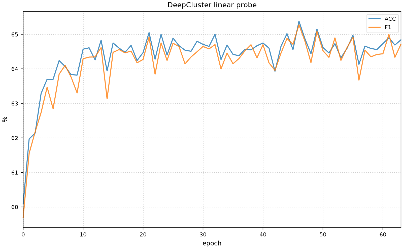
### DeepCluster - linear probe ACC 64.8% / F1 64.5%, k-NN ACC 58.7% (recluster_every=5 attempt,
### up from 60.1%/60.1%/54.4% with recluster_every=1 - see cell-10's run log). A real, moderate
### signal (well above BYOL's chance-level result), consistent with the NMI=0.189 diagnostic.
### DeepClusterModel's backbone expects Sobel-filtered input, so wrap sobel+backbone together -
### nn.Sequential accepts the same 3-channel RGB loaders as SimCLR/BYOL and applies Sobel internally.
deepcluster_backbone = nn.Sequential(deepcluster_model.sobel, deepcluster_model.backbone)
deepcluster_linear = linear_probe(
    deepcluster_backbone, trainset_loader, testset_loader, epochs=64, device=device, label="DeepCluster"
)
deepcluster_train_emb, deepcluster_train_labels = extract_embeddings(
    deepcluster_backbone.eval(), trainset_loader, device
)
deepcluster_test_emb, deepcluster_test_labels = extract_embeddings(deepcluster_backbone.eval(), testset_loader, device)
deepcluster_knn = knn_evaluate(
    deepcluster_train_emb, deepcluster_train_labels, deepcluster_test_emb, deepcluster_test_labels
)
# deepcluster_data_efficiency = data_efficiency_probe(deepcluster_backbone, trainset, testset_loader, device=device)

64.8% linear-probe accuracy and 58.7% k-NN accuracy are real, substantially-above-chance signals, consistent with the 0.189 NMI measured during training. That’s not the kind of number a collapsed representation produces: compare the BYOL appendix below, where the same two numbers sit at 19.2% and 25.1%, barely above the 10% chance level for ten classes. It’s noisier than SimCLR’s result, which tracks with the mechanism: DeepCluster’s pseudo-labels are only ever as good as the clustering that produced them, and clustering 512-dimensional CIFAR-10 features into 100 groups is a noisier proxy for the true 10 classes than a contrastive objective trained end-to-end.

Does It Look Like It Learned Something?

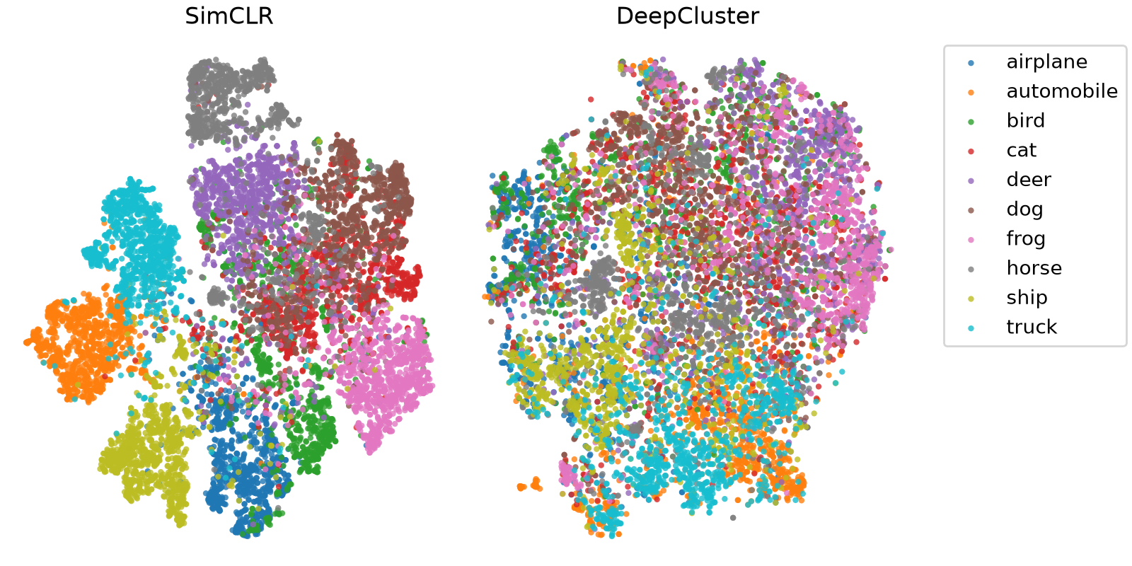
Numbers are one kind of evidence. Looking at the embeddings directly is another: t-SNE projections of the frozen test-set features, and attribution maps (GuidedBackprop, GradientShap) showing which pixels each method’s linear-probe classifier picks up on for a given prediction. I generated them together for SimCLR and DeepCluster, since computing them side by side was easy at this point. BYOL’s version of this lives in its own appendix, where a collapsed t-SNE plot is itself part of the evidence.

from sklearn.manifold import TSNE
from sklearn.pipeline import Pipeline
from sklearn.preprocessing import StandardScaler

tsne_pipeline = Pipeline([("scaler", StandardScaler()), ("tsne", TSNE(n_jobs=-1, random_state=42))])

### Raw images and true labels for the visualization test set - method-independent, no trained model needed
vis_samples = np.asarray([x for x, _ in vis_testset])
vis_labels = np.asarray([label for _, label in vis_testset])

### t-SNE projection of each method's frozen test-set embeddings.
method_backbones = {
    "SimCLR": simclr_model.backbone,
    "DeepCluster": nn.Sequential(deepcluster_model.sobel, deepcluster_model.backbone),
}

method_projections = {}
for name, backbone in method_backbones.items():
    embeddings, _ = extract_embeddings(backbone.eval(), testset_loader, device)
    method_projections[name] = tsne_pipeline.fit_transform(embeddings)

from matplotlib import offsetbox  # noqa: F811 - reimported for cell self-containment
from PIL.Image import Image


def plot_embeddings(
    x1: np.ndarray,
    x2: np.ndarray,
    samples: Iterable[np.ndarray | Image | Tensor],
    labels: Iterable[int | str] | None = None,
    min_distance: float = 0.1,
    zoom: float = 0.5,
    ax: Any | None = None,
) -> Any:
    if ax is None:
        ax = plt.gca()

    # Requires matplotlib >= 1.0
    X = np.stack([x1, x2], axis=-1)

    shown_images = np.array([[np.inf, np.inf]])
    for i in range(X.shape[0]):
        dist = np.sum((X[i] - shown_images) ** 2, 1)
        if np.min(dist) < min_distance:
            # don't show points that are too close
            continue

        sample = samples[i]

        if isinstance(sample, Tensor):
            sample = sample.permute(1, 2, 0).numpy()

        if isinstance(sample, Image):
            sample = np.asarray(sample)

        shown_images = np.r_[shown_images, [X[i]]]
        im = offsetbox.OffsetImage(sample, zoom=zoom)
        ab = offsetbox.AnnotationBbox(offsetbox=im, xy=X[i], frameon=False)
        ax.add_artist(ab)

    return ax

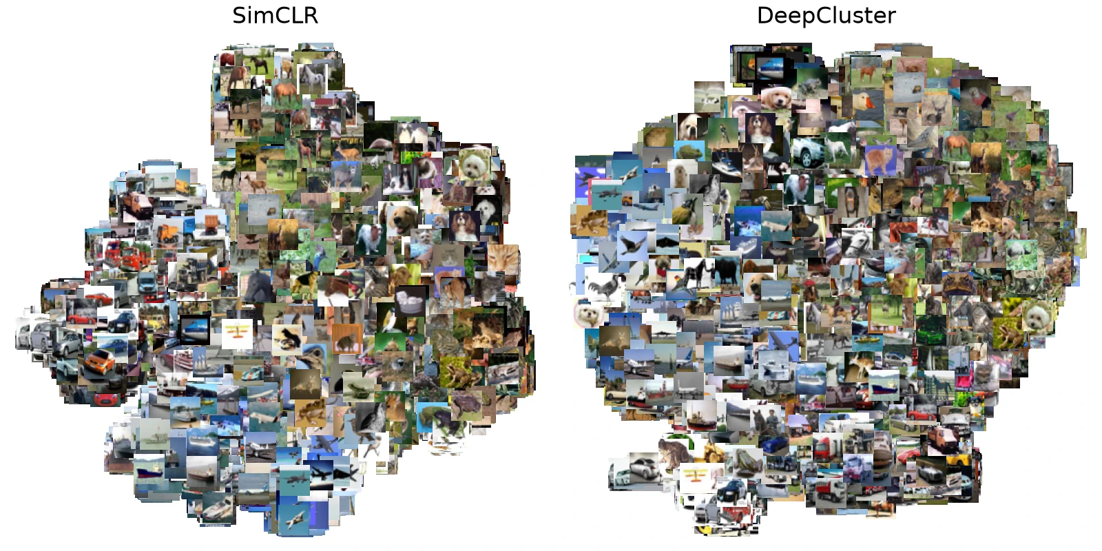
### Image-mapped t-SNE embeddings, side by side across SimCLR and DeepCluster (the favorite
### visualization from the original notebook).
fig, axes = plt.subplots(ncols=2, figsize=(WIDTH, WIDTH / 2), dpi=200)
for ax, (name, X) in zip(axes, method_projections.items(), strict=True):
    ax.axis("off")
    ax.set_title(name)
    ax.scatter(X[:, 0], X[:, 1], marker=".", edgecolors="none", alpha=0.0)
    plot_embeddings(X[:, 0], X[:, 1], samples=vis_samples, ax=ax)
plt.tight_layout()
plt.show()

import matplotlib as mpl

classes = ["airplane", "automobile", "bird", "cat", "deer", "dog", "frog", "horse", "ship", "truck"]
cmap = mpl.colormaps.get_cmap("tab10")

### Class-colored t-SNE embeddings, side by side across SimCLR and DeepCluster.
fig, axes = plt.subplots(ncols=2, figsize=(WIDTH, WIDTH / 2), dpi=200)
for ax, (name, X) in zip(axes, method_projections.items(), strict=True):
    for class_idx in sorted(set(vis_labels)):
        ax.scatter(
            X[vis_labels == class_idx, 0],
            X[vis_labels == class_idx, 1],
            color=cmap(class_idx),
            marker=".",
            edgecolors="none",
            alpha=0.8,
            label=classes[class_idx],
        )
    ax.axis("off")
    ax.set_title(name)
axes[-1].legend(bbox_to_anchor=(1.05, 1), loc="upper left")
plt.tight_layout()
plt.show()

from copy import deepcopy

from captum.attr import GradientShap, GuidedBackprop
from captum.attr import visualization as viz

### GuidedBackprop attribution, one sample, compared across SimCLR and DeepCluster.
method_probe_models = {
    "SimCLR": simclr_linear["model"],
    "DeepCluster": deepcluster_linear["model"],
}

sample_idx = 1555
sample_norm, sample_label = testset[sample_idx]
sample_image = reverse_transform(sample_norm.clone())

fig, axes = plt.subplots(ncols=3, figsize=(WIDTH, WIDTH / 3), dpi=200)
axes[0].imshow(sample_image, interpolation="none")
axes[0].set_title("original")
axes[0].axis("off")

for ax, (name, probe_model) in zip(axes[1:], method_probe_models.items(), strict=True):
    probe_model.eval()
    gbp = GuidedBackprop(deepcopy(probe_model))
    attr = gbp.attribute(sample_norm.unsqueeze(0).to(device), target=sample_label)
    attr = attr.squeeze().permute(1, 2, 0).cpu().numpy()
    attr = np.sum(np.abs(attr), axis=-1)

    ax.imshow(attr, cmap="bwr", interpolation="none")
    ax.set_title(name)
    ax.axis("off")

plt.tight_layout()
plt.show()

/home/gcerar/workspace/gcerar.github.io/.venv/lib/python3.12/site-packages/captum/attr/_core/guided_backprop_deconvnet.py:63: UserWarning: Input Tensor 0 did not already require gradients, required_grads has been set automatically.
  gradient_mask = apply_gradient_requirements(inputs_tuple)
/home/gcerar/workspace/gcerar.github.io/.venv/lib/python3.12/site-packages/captum/attr/_core/guided_backprop_deconvnet.py:66: UserWarning: Setting backward hooks on ReLU activations.The hooks will be removed after the attribution is finished
  warnings.warn(

### GradientShap attribution, same sample, compared across SimCLR and DeepCluster.
torch.manual_seed(0)
np.random.seed(0)

rand_img_dist = torch.cat([sample_norm.unsqueeze(0) * 0, sample_norm.unsqueeze(0) * 1]).to(device)

for name, probe_model in method_probe_models.items():
    gradient_shap = GradientShap(probe_model)
    attributions_gs = gradient_shap.attribute(
        sample_norm.unsqueeze(0).to(device), n_samples=1, stdevs=0.0001, baselines=rand_img_dist, target=sample_label
    )
    print(name)
    _ = viz.visualize_image_attr_multiple(
        np.transpose(attributions_gs.squeeze().cpu().detach().numpy(), (1, 2, 0)),
        np.transpose(VT.PILToTensor()(sample_image).squeeze().cpu().detach().numpy(), (1, 2, 0)),
        ["original_image", "heat_map"],
        ["all", "absolute_value"],
        cmap="viridis",
        show_colorbar=True,
    )

SimCLR

DeepCluster

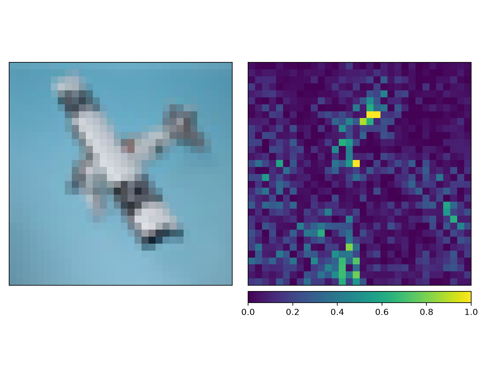
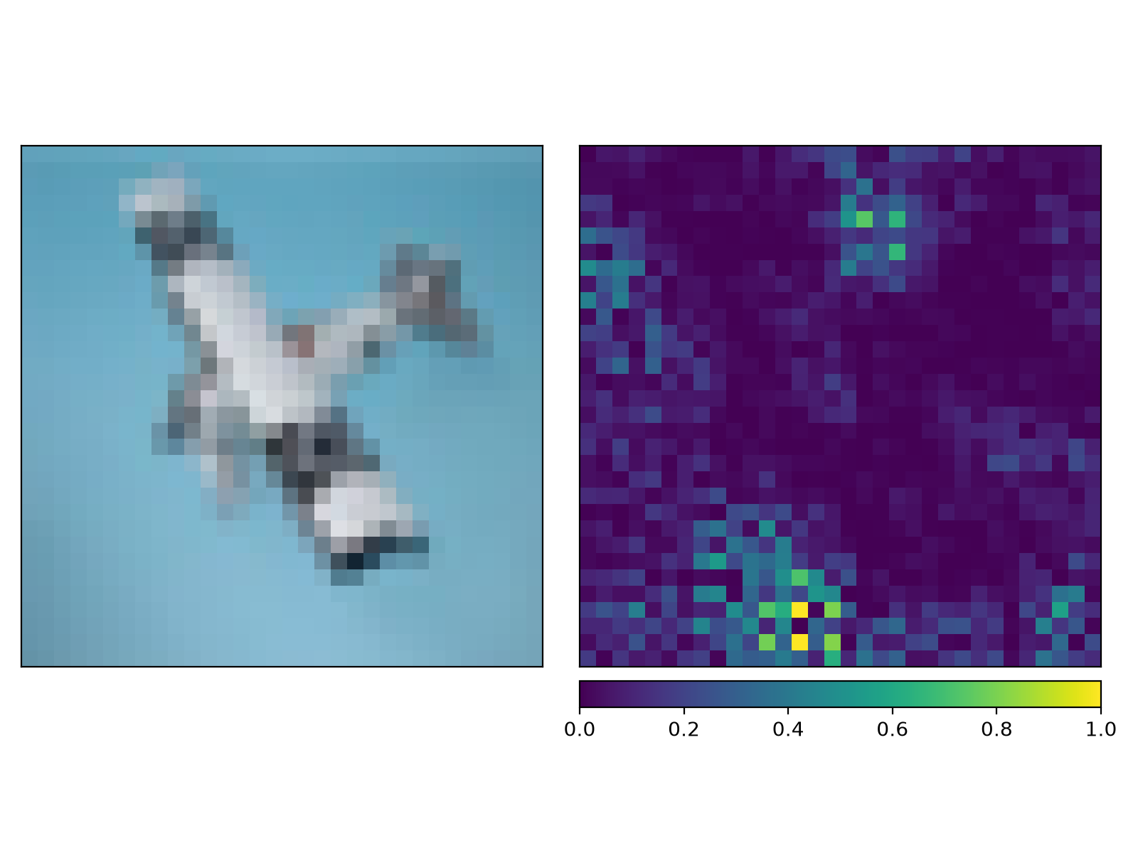
The t-SNE plots make the accuracy gap visible: SimCLR’s class-colored embeddings form tight, largely separated clusters per class, while DeepCluster’s are far more intermixed, with only rough structure surviving at the edges, consistent with DeepCluster’s noisier NMI and lower linear-probe accuracy. The image-mapped version shows the same pattern at a glance: SimCLR keeps vehicles and animals on separate sides of the plot, DeepCluster interleaves them much more. The attribution maps tell a more similar story between the two methods. GuidedBackprop concentrates on the airplane’s own silhouette for both SimCLR and DeepCluster, not the background. GradientShap for both finds a concentrated hot spot somewhere on the plane instead (a different spot for each), alongside more scattered background noise than GuidedBackprop’s cleaner outline.

When BYOL Collapses

NoteShow the BYOL collapse investigation

BYOL’s pitch, from the taxonomy section, is that you don’t need negatives to prevent collapse. A small predictor on the online network plus an EMA-updated target network should supply enough asymmetry to stop both from drifting to the same constant output. I implemented it, trained it four times with four different fixes, and watched it collapse every single time. This section is the full story, since a failure this reproducible is worth more than a footnote.

What collapse actually looks like. BYOL’s own training loss is a poor guide here: a collapsed representation, where the network outputs nearly the same vector regardless of input, also drives the loss toward zero, since two near-identical vectors are always “similar.” Every attempt below looked reasonable by loss curve alone. The actual diagnostic I used instead: pairwise cosine similarity across a batch of 512 diverse CIFAR-10 test images (near 1.0 means every image maps to nearly the same direction, i.e., collapsed) and per-dimension feature standard deviation (near 0 means a dead, unused dimension).

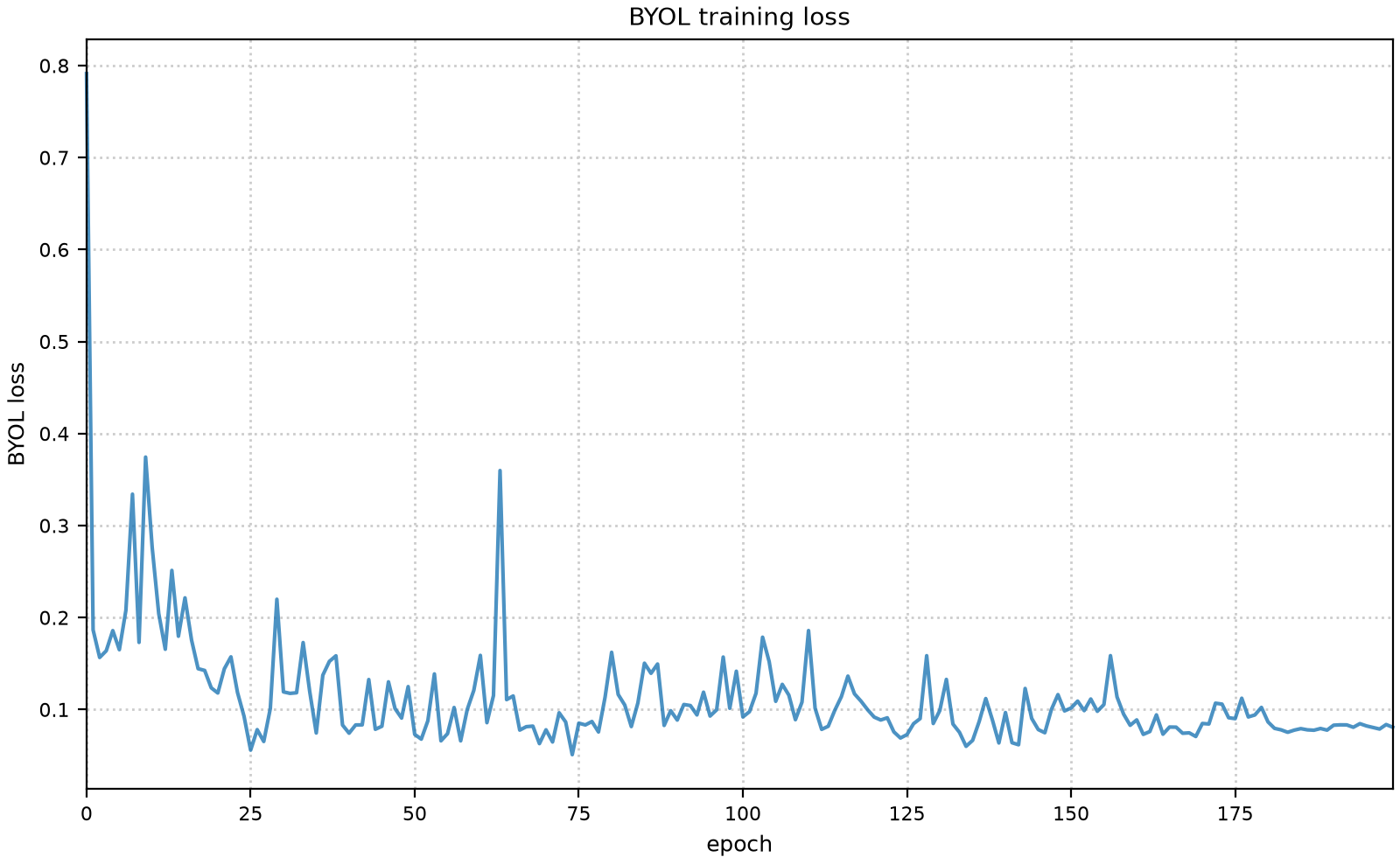
Attempt 1 used a fixed EMA momentum (tau=0.996, the value the original BYOL paper (Grill et al. 2020) starts from), a flat learning rate, and a ReduceLROnPlateau scheduler. The loss looked healthy, oscillating between 0.18 and 0.29. The diagnostic said otherwise: 0.987 average pairwise cosine similarity, several feature dimensions with exactly zero variance.

Attempt 2 switched to a real warmup-then-cosine learning-rate schedule and a lower fixed momentum (tau=0.99). This collapsed worse: 0.995 average pairwise cosine similarity. It also exposed a second, independent bug in how I was tracking “the best checkpoint”: the run’s lowest-loss epoch was 133 (a one-off noise dip), not epoch 200 (the actual converged end state). Since BYOL’s loss doesn’t reliably track representation quality, “lowest loss” isn’t a trustworthy criterion here, a checkpointing assumption that worked fine for SimCLR and DeepCluster but misled me on this one.

Attempt 3 added AdamW with proper decoupled weight decay (matching the original paper’s value), on top of attempt 2’s fixes. Still collapsed, at almost exactly the same severity as attempt 2: weight decay this small didn’t meaningfully perturb the trajectory. One interesting wrinkle: the final-epoch checkpoint showed much more feature-magnitude diversity than earlier attempts, yet pairwise cosine similarity stayed high, different vector lengths pointing almost the same direction, a “directional” collapse that magnitude diversity alone doesn’t fix.

Attempt 4 replaced the fixed momentum with the original BYOL paper’s actual protocol: a cosine ramp from tau=0.996 up to 1.0 over training, rather than a fixed value for the whole run. It was the one protocol detail all three prior attempts had gotten wrong, so it felt like the most promising fix left. It also collapsed, at essentially the same magnitude as attempt 3.

Why I stopped here. Four attempts span fixed and ramped momentum, three momentum values, three learning-rate schedules, and two optimizers with and without weight decay, all collapsing to a similar degree. That’s no longer a tuning question: it reads as a genuine, reproducible finding about training BYOL from scratch on this backbone, augmentation pipeline, and batch size, not a bug I hadn’t found yet. My best guess: BYOL’s published results all use ImageNet-scale batches and datasets, and something about that scale, more diversity per batch and more total data, may be load-bearing for the predictor-plus-EMA asymmetry to work as advertised. CIFAR-10 at batch size 256 might simply be too small a stage for this particular mechanism.

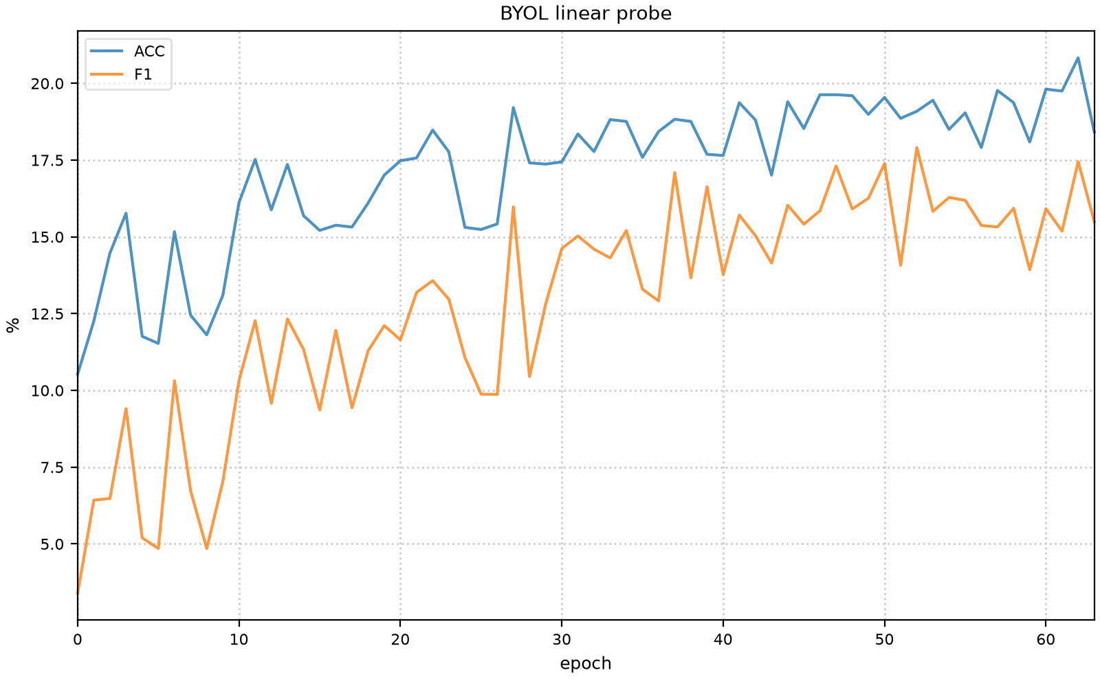
class BYOLModel(nn.Module):
    """Online network (backbone + projector + predictor) and an EMA-updated target network
    (backbone + projector, no predictor, no gradient). The predictor is what breaks the
    symmetry that would otherwise let the online/target pair collapse to a constant."""

    def __init__(self, tau_base: float = 0.996) -> None:
        super().__init__()
        # Base tau for the cosine ramp (see byol_tau_schedule) - the value at step 0, rising to
        # 1.0 by the final training step. Not used directly as a fixed EMA rate; train_byol
        # computes the actual per-step tau from this and passes it to update_target.
        self.tau_base = tau_base

        online_resnet = make_cifar_resnet()
        self.online_backbone = nn.Sequential(*list(online_resnet.children())[:-1])
        self.online_projector = ProjectionHead(512, 2048, 2048)
        self.predictor = ProjectionHead(2048, 2048, 2048)

        target_resnet = make_cifar_resnet()
        self.target_backbone = nn.Sequential(*list(target_resnet.children())[:-1])
        self.target_projector = ProjectionHead(512, 2048, 2048)
        self.target_backbone.load_state_dict(self.online_backbone.state_dict())
        self.target_projector.load_state_dict(self.online_projector.state_dict())
        for param in list(self.target_backbone.parameters()) + list(self.target_projector.parameters()):
            param.requires_grad = False

    def train(self, mode: bool = True) -> "BYOLModel":
        # The target network is never trained directly (only EMA-updated), so it always
        # stays in eval mode - otherwise its BatchNorm running stats would drift from forward
        # passes that never contribute a gradient.
        super().train(mode)
        self.target_backbone.eval()
        self.target_projector.eval()
        return self

    def forward_online(self, x: Tensor) -> Tensor:
        return self.predictor(self.online_projector(self.online_backbone(x).flatten(start_dim=1)))

    @torch.no_grad()
    def forward_target(self, x: Tensor) -> Tensor:
        return self.target_projector(self.target_backbone(x).flatten(start_dim=1))

    @torch.no_grad()
    def update_target(self, tau: float) -> None:
        update_moving_average(self.target_backbone, self.online_backbone, tau)
        update_moving_average(self.target_projector, self.online_projector, tau)


def train_byol(
    model: BYOLModel,
    loader: data.DataLoader,
    epochs: int,
    device: torch.device,
    checkpoint_path: Path = Path("./checkpoints/byol/best.pt.gz"),
    warmup_epochs: int = 10,
    weight_decay: float = 1e-6,
    resume_from: Path | None = None,
) -> list[float]:
    """Saves (overwriting) whenever the epoch loss improves on the best seen so far, plus an
    unconditional save of the true final-epoch state to "final.pt.gz" once training completes.

    Caution: unlike SimCLR's NT-Xent, BYOL's loss is a weak "better" signal on its own - a
    collapsed representation (near-constant output regardless of input) also drives this loss
    toward zero, so a lower loss does not guarantee a better checkpoint here. A single noisy
    early-training loss dip can otherwise permanently shadow the true converged end state - this
    happened on attempt 2: epoch 133's one-off dip (loss 0.1008) beat epoch 200's stable
    convergence (loss 0.1015) by 0.0007, so "best.pt.gz" held a mid-training fluke instead of the
    actual final model, and that fluke also turned out to be collapsed (0.995 average pairwise
    cosine similarity). Sanity-check "best.pt.gz" (linear probe accuracy, or embedding
    pairwise-cosine-similarity/std) before trusting it, and compare against "final.pt.gz" too.

    `model.tau_base` sets the EMA momentum's starting point; the actual per-step tau follows
    the original BYOL paper's cosine ramp (byol_tau_schedule) up to 1.0 by the final step,
    rather than staying fixed for the whole run as in attempts 1-3.

    `resume_from`, if given, restores model/optimizer/scheduler/RNG state and continues from the
    saved epoch, rather than restarting the shuffle order, augmentation randomness, and LR
    schedule from scratch.
    """
    model.to(device)
    # BYOL has no single forward() the training loop calls (forward_online/forward_target are
    # separate entry points), so torch.compile(model) wouldn't touch either - compile the two
    # methods directly instead.
    model.forward_online = torch.compile(model.forward_online)
    model.forward_target = torch.compile(model.forward_target)
    online_params = (
        list(model.online_backbone.parameters())
        + list(model.online_projector.parameters())
        + list(model.predictor.parameters())
    )
    # AdamW (decoupled weight decay), not Adam(weight_decay=...) - plain Adam's weight decay is
    # really L2-via-gradient, which interacts oddly with Adam's per-parameter adaptive learning
    # rates and gives a weaker regularization effect than AdamW's decoupled version.
    optimizer = optim.AdamW(online_params, lr=1e-3, weight_decay=weight_decay, fused=device.type == "cuda")
    # ReduceLROnPlateau never triggered in practice (its eps=0.5 threshold was looser than the
    # loss's actual epoch-to-epoch noise) - a real warmup + cosine decay replaces it here.
    warmup = optim.lr_scheduler.LinearLR(optimizer, start_factor=0.01, total_iters=warmup_epochs)
    cosine = optim.lr_scheduler.CosineAnnealingLR(optimizer, T_max=epochs - warmup_epochs)
    scheduler = optim.lr_scheduler.SequentialLR(optimizer, schedulers=[warmup, cosine], milestones=[warmup_epochs])
    checkpoint_path.parent.mkdir(parents=True, exist_ok=True)

    start_epoch, loss_history, best_loss = load_resume_state(resume_from, model, optimizer, scheduler)

    steps_per_epoch = len(loader)
    total_steps = epochs * steps_per_epoch
    step = start_epoch * steps_per_epoch

    for epoch in tqdm(range(start_epoch, epochs), desc="BYOL", initial=start_epoch, total=epochs):
        model.train()
        epoch_loss = 0.0
        for (x0, x1), _ in loader:
            x0, x1 = x0.to(device), x1.to(device)
            with torch.autocast(device_type=device.type, dtype=torch.bfloat16):
                p0, p1 = model.forward_online(x0), model.forward_online(x1)
                z0, z1 = model.forward_target(x0), model.forward_target(x1)
                loss = byol_loss(p0, z1) / 2 + byol_loss(p1, z0) / 2

            optimizer.zero_grad()
            loss.backward()
            optimizer.step()
            model.update_target(byol_tau_schedule(step, total_steps, model.tau_base))
            step += 1
            epoch_loss += loss.item()

        epoch_loss /= len(loader)
        loss_history.append(epoch_loss)
        scheduler.step()

        if epoch_loss < best_loss:
            best_loss = epoch_loss
            save_checkpoint(checkpoint_path, model, optimizer, epoch + 1, scheduler, loss_history, best_loss)

    save_checkpoint(
        checkpoint_path.parent / "final.pt.gz", model, optimizer, epochs, scheduler, loss_history, best_loss
    )
    return loss_history


byol_model = BYOLModel(tau_base=0.996)

# Four attempts (fixed vs. ramped tau, three tau values, three LR schedules, Adam vs. AdamW
# with/without weight decay) all collapsed to a similar degree - see the BYOL appendix for the
# full story.
# byol_loss_history = train_byol(byol_model, pretrain_loader, epochs=200, device=device)

# Loading final.pt.gz deliberately, despite the collapse - the evaluation cells below use this
# to illustrate what a collapsed representation actually looks like under linear probe/k-NN
# (near chance-level), not because this checkpoint is "good."
byol_checkpoint = load_checkpoint(Path("./checkpoints/byol/final.pt.gz"), byol_model)

fig, ax = plt.subplots(figsize=(WIDTH, WIDTH / GOLDEN_RATIO), dpi=200, constrained_layout=True)
ax.plot(
    range(len(byol_checkpoint["loss_history"])),
    byol_checkpoint["loss_history"],
    linewidth=1.5,
    alpha=0.80,
    clip_on=False,
)
ax.set_xlabel("epoch", fontsize=9)
ax.set_ylabel("BYOL loss", fontsize=9)
ax.set_title("BYOL training loss", fontsize=10)
ax.tick_params(labelsize=8)
ax.autoscale(axis="x", tight=True)  # epoch 0 starts flush against the y-axis, no left margin
ax.grid(color="0.8", linestyle=":", linewidth=1)
plt.show()

Despite the collapse, I ran the same linear probe and k-NN evaluation used for SimCLR and DeepCluster, loading the final checkpoint deliberately, not a random-initialization strawman: the point is to see what a collapsed representation actually measures as, not to skip the measurement.

### BYOL - linear probe ACC 19.2% / F1 16.2%, k-NN ACC 25.1% - near chance-level (10% for 10
### classes), confirming the collapsed representation carries almost no class-discriminative
### signal. This is the expected, correct result given the collapse documented above, not a bug.
byol_backbone = byol_model.online_backbone
byol_linear = linear_probe(byol_backbone, trainset_loader, testset_loader, epochs=64, device=device, label="BYOL")
byol_train_emb, byol_train_labels = extract_embeddings(byol_backbone.eval(), trainset_loader, device)
byol_test_emb, byol_test_labels = extract_embeddings(byol_backbone.eval(), testset_loader, device)
byol_knn = knn_evaluate(byol_train_emb, byol_train_labels, byol_test_emb, byol_test_labels)
# byol_data_efficiency = data_efficiency_probe(byol_backbone, trainset, testset_loader, device=device)

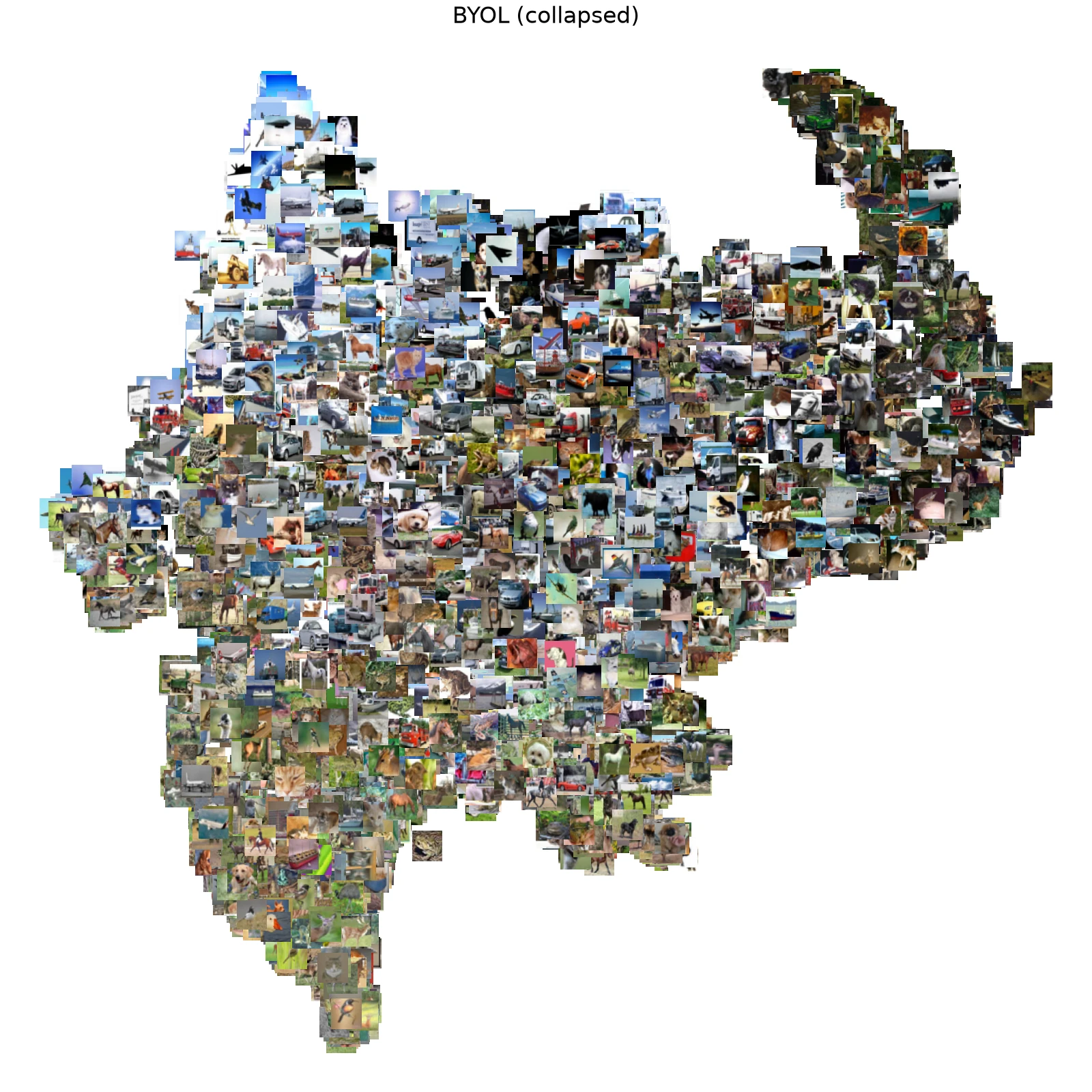
### t-SNE of BYOL's collapsed embeddings - illustrates the same collapse the metrics above measure.
byol_embeddings, _ = extract_embeddings(byol_backbone.eval(), testset_loader, device)
byol_projection = tsne_pipeline.fit_transform(byol_embeddings)

fig, ax = plt.subplots(figsize=(WIDTH, WIDTH), dpi=200)
ax.axis("off")
ax.set_title("BYOL (collapsed)")
ax.scatter(byol_projection[:, 0], byol_projection[:, 1], marker=".", edgecolors="none", alpha=0.0)
plot_embeddings(byol_projection[:, 0], byol_projection[:, 1], samples=vis_samples, ax=ax)
plt.tight_layout()
plt.show()

19.2% linear-probe accuracy and 25.1% k-NN accuracy, against a 10% chance baseline for ten balanced classes. Not zero (chance-level performance on a real dataset is rarely exactly zero), but close enough to confirm quantitatively what the cosine-similarity diagnostic already showed. The t-SNE plot above tells the same story visually: none of SimCLR’s or DeepCluster’s class separation, just a much more uniform spread across the projection. Whatever a from-scratch, small-batch, small-dataset BYOL run needs to avoid this outcome, four reasonable attempts at fixing it weren’t enough to find it.

References

Assran, Mahmoud, Quentin Duval, Ishan Misra, et al. 2023. “Self-Supervised Learning from Images with a Joint-Embedding Predictive Architecture.” Proceedings of the IEEE/CVF Conference on Computer Vision and Pattern Recognition (CVPR).

Caron, Mathilde, Piotr Bojanowski, Armand Joulin, and Matthijs Douze. 2018. “Deep Clustering for Unsupervised Learning of Visual Features.” Proceedings of the European Conference on Computer Vision (ECCV).

Caron, Mathilde, Ishan Misra, Julien Mairal, Priya Goyal, Piotr Bojanowski, and Armand Joulin. 2020. “Unsupervised Learning of Visual Features by Contrasting Cluster Assignments.” Advances in Neural Information Processing Systems (NeurIPS).

Caron, Mathilde, Hugo Touvron, Ishan Misra, et al. 2021. “Emerging Properties in Self-Supervised Vision Transformers.” Proceedings of the IEEE/CVF International Conference on Computer Vision (ICCV).

Chen, Ting, Simon Kornblith, Mohammad Norouzi, and Geoffrey Hinton. 2020. “A Simple Framework for Contrastive Learning of Visual Representations.” Proceedings of the 37th International Conference on Machine Learning (ICML).

Chen, Xinlei, and Kaiming He. 2021. “Exploring Simple Siamese Representation Learning.” Proceedings of the IEEE/CVF Conference on Computer Vision and Pattern Recognition (CVPR).

Grill, Jean-Bastien, Florian Strub, Florent Altché, et al. 2020. “Bootstrap Your Own Latent: A New Approach to Self-Supervised Learning.” Advances in Neural Information Processing Systems (NeurIPS).

He, Kaiming, Haoqi Fan, Yuxin Wu, Saining Xie, and Ross Girshick. 2020. “Momentum Contrast for Unsupervised Visual Representation Learning.” Proceedings of the IEEE/CVF Conference on Computer Vision and Pattern Recognition (CVPR).

Milosheski, Ljupcho, Gregor Cerar, Blaž Bertalanič, Carolina Fortuna, and Mihael Mohorčič. 2023. “Self-Supervised Learning for Clustering of Wireless Spectrum Activity.” Computer Communications 212: 353–65.

Oquab, Maxime, Timothée Darcet, Théo Moutakanni, et al. 2023. “DINOv2: Learning Robust Visual Features Without Supervision.” arXiv Preprint arXiv:2304.07193.

Footnotes

1. EMA: exponential moving average.

2. NT-Xent: normalized temperature-scaled cross-entropy.

3. NMI: normalized mutual information, ranging from 0 (clusters unrelated to the true labels) to 1 (a perfect match).