Generative Adversarial Networks

Abstract

Generative Adversarial Networks (GANs) represent an innovative class of unsupervised neural networks that have revolutionized the field of artificial intelligence. Eager to learn how they work, I’ve implemented foundational “vanilla” GAN and its more complex counterpart, the Deep Convolutional GAN (DCGAN), from scratch. I’ve put them on a test run on MNIST Digits and Fashion toy datasets.

Introduction

Generative Adversarial Networks (GANs) were introduced in Generative Adversarial Networks (Goodfellow et al. 2014) and consist of two separate neural networks: the generator (creates data) and the discriminator (evaluates data authenticity). The generator aims to fool the discriminator by producing realistic data, while the discriminator tries to differentiate real from fake. Over iterations, the generator’s data becomes more convincing.

As an analogy, consider two kids, one drawing counterfeit money (“Generator”) and another assessing its realism (“Discriminator”). Over time, the counterfeit drawings become increasingly convincing.

Vanilla GAN

The most fundamental variant of GAN is the “vanilla” GAN, where “vanilla” signifies the model in its original and most straightforward form rather than a flavor. To better understand its mechanism, I’ve illustrated its structure on Figure 1.

Figure 1: GAN architecture

• Generator \(G(z; w_g)\) takes random noise \(z\) as input and produces fabricated data \(x_f\).
  • \(z\) represents the input vector, a noise vector from the Gaussian distribution.
  • \(w_g\) denotes generator neural network weights.
  • \(x_f\) is a fabricated data sample meant for the discriminator.
• Discriminator \(D(x; w_d)\) differentiates between real and generated data.
  • \(x\) represents input vectors, which come from either a real dataset (\(x_r \sim p_\textrm{data}(x)\)) or from the set of fabricated samples (\(x_f = G(z \sim p_z(z); w_g)\)).
  • \(w_d\) denotes discriminator neural network weights.

Objective Function

The interaction between the Generator and the Discriminator can be quantified by their objective or loss functions:

• Discriminator’s Objective: For real data \(x\), \(D\) wants \(D(x)\) near \(1\). For generated data \(G(z)\), it targets \(D(G(z))\) close to \(0\). Its objective is:

\[ \mathcal{L}(D) = \log(D(x)) + \log(1 - D(G(z))). \]

• Generator’s Objective: \(G\) aims for \(D(G(z))\) to approach \(1\), given by:

\[ \mathcal{L}(G) = \log(1 - D(G(z))) \]

Both \(G\) and \(D\) continuously improve to outperform each other in this game.

Minimax Game in GANs

Vanilla GANs are structured around the minimax game from game theory:

\[ \min_{G}\max_{D} \mathcal{L}(D, G) = \log(D(x)) + \log(1 - D(G(z))) \]

In essence:

• Discriminator: Maximizes its capacity to differentiate real data from generated.
• Generator: Minimizes the discriminator’s success rate by producing superior forgeries.

The iterative competition refines both, targeting a proficient Generator and a perceptive Discriminator.

Prepare Components

In the upcoming sections, I’ll do the following steps to prepare the development environment:

• Import necessary libraries, primarily PyTorch and Matplotlib.
• Define constants, including project path and seed, for consistency.
• Determine the computational device (e.g., GPU).
• Provide a weight initialization helper function.

from collections.abc import Callable, Sequence
from pathlib import Path
from typing import Any, Final

import joblib
import numpy as np
from matplotlib import pyplot as plt

%config InlineBackend.figure_formats = {'retina', 'png'}

import torch
from torch import Tensor, nn, optim
from torch.utils.data import ConcatDataset, DataLoader, Dataset
from torchinfo import summary
from torchvision import transforms as T
from torchvision.utils import make_grid
from tqdm import tqdm

SEED: Final[int] = 42

PROJECT_PATH = Path(".").resolve()
FIGURE_PATH = PROJECT_PATH / "figures"
DATASET_PATH = Path.home() / "datasets"

# Common constants for all experiments
IMG_DIM: Final[tuple[int, int, int]] = (1, 28, 28)

device = torch.device("cpu")

if torch.cuda.is_available():
    device = torch.device("cuda")

def weights_init(net: nn.Module) -> None:
    for m in net.modules():
        if isinstance(m, nn.Conv2d | nn.ConvTranspose2d):
            nn.init.normal_(m.weight, 0.0, 0.02)
            if m.bias is not None:
                nn.init.constant_(m.bias, 0.0)

        elif isinstance(m, nn.BatchNorm1d | nn.BatchNorm2d):
            nn.init.normal_(m.weight, 1.0, 0.02)
            if m.bias is not None:
                nn.init.constant_(m.bias, 0.0)

        elif isinstance(m, nn.Linear):
            nn.init.normal_(m.weight, 0, 0.02)
            if m.bias is not None:
                nn.init.constant_(m.bias, 0.0)

Generator

The Generator in GANs acts as an artist, crafting data.

• Input: Takes random noise, typically from a standard normal distribution.
• Architecture: Uses dense layers, progressively increasing data dimensions.
• Output: Reshapes data to desired format (e.g., image). Often uses “tanh” for activation.
• Objective: Generate data indistinguishable from real by the Discriminator.

class Generator(nn.Module):
    def __init__(self, out_dim: Sequence[int], nz: int = 100, ngf: int = 256, alpha: float = 0.2):
        """
        :param out_dim: output image dimension / shape
        :param nz: size of the latent z vector $z$
        :param ngf: size of feature maps (units in the hidden layers) in the generator
        :param alpha: negative slope of leaky ReLU activation
        """
        super().__init__()
        self.out_dim = out_dim
        self.model = nn.Sequential(
            nn.Linear(nz, ngf),
            nn.LeakyReLU(alpha, inplace=True),
            nn.Linear(ngf, 2 * ngf),
            nn.LeakyReLU(alpha, inplace=True),
            nn.Linear(2 * ngf, 4 * ngf),
            nn.LeakyReLU(alpha, inplace=True),
            nn.Linear(4 * ngf, int(np.prod(self.out_dim))),
            nn.Tanh(),
        )

    def forward(self, x: Tensor) -> Tensor:
        x = self.model(x)
        x = torch.reshape(x, (x.size(0), *self.out_dim))
        return x


summary(Generator(out_dim=(1, 28, 28)), input_size=[128, 100])

==========================================================================================
Layer (type:depth-idx)                   Output Shape              Param #
==========================================================================================
Generator                                [128, 1, 28, 28]          --
├─Sequential: 1-1                        [128, 784]                --
│    └─Linear: 2-1                       [128, 256]                25,856
│    └─LeakyReLU: 2-2                    [128, 256]                --
│    └─Linear: 2-3                       [128, 512]                131,584
│    └─LeakyReLU: 2-4                    [128, 512]                --
│    └─Linear: 2-5                       [128, 1024]               525,312
│    └─LeakyReLU: 2-6                    [128, 1024]               --
│    └─Linear: 2-7                       [128, 784]                803,600
│    └─Tanh: 2-8                         [128, 784]                --
==========================================================================================
Total params: 1,486,352
Trainable params: 1,486,352
Non-trainable params: 0
Total mult-adds (Units.MEGABYTES): 190.25
==========================================================================================
Input size (MB): 0.05
Forward/backward pass size (MB): 2.64
Params size (MB): 5.95
Estimated Total Size (MB): 8.63
==========================================================================================

Discriminator

The Discriminator is GAN’s evaluator, distinguishing real from fake data.

• Input: Takes either real data samples or those from the Generator.
• Architecture: Employs dense layers for binary classification of the input.
• Output: Produces raw logits (unbounded scores) evaluated by BCEWithLogitsLoss, which applies an implicit sigmoid for numerical stability.
• Objective: Recognize real data and identify fake data from the Generator.

class Discriminator(nn.Module):
    def __init__(self, input_dim: Sequence[int], ndf: int = 128, alpha: float = 0.2):
        super().__init__()
        self.model = nn.Sequential(
            nn.Linear(int(np.prod(input_dim)), 4 * ndf),
            nn.LeakyReLU(alpha, inplace=True),
            nn.Dropout(0.3),
            nn.Linear(4 * ndf, 2 * ndf),
            nn.LeakyReLU(alpha, inplace=True),
            nn.Dropout(0.3),
            nn.Linear(2 * ndf, ndf),
            nn.LeakyReLU(alpha, inplace=True),
            nn.Dropout(0.3),
            nn.Linear(ndf, 1),
        )

    def forward(self, x: Tensor) -> Tensor:
        x = torch.reshape(x, (x.size(0), -1))
        return self.model(x)


summary(Discriminator(input_dim=(1, 28, 28)), input_size=[128, 1, 28, 28])

==========================================================================================
Layer (type:depth-idx)                   Output Shape              Param #
==========================================================================================
Discriminator                            [128, 1]                  --
├─Sequential: 1-1                        [128, 1]                  --
│    └─Linear: 2-1                       [128, 512]                401,920
│    └─LeakyReLU: 2-2                    [128, 512]                --
│    └─Dropout: 2-3                      [128, 512]                --
│    └─Linear: 2-4                       [128, 256]                131,328
│    └─LeakyReLU: 2-5                    [128, 256]                --
│    └─Dropout: 2-6                      [128, 256]                --
│    └─Linear: 2-7                       [128, 128]                32,896
│    └─LeakyReLU: 2-8                    [128, 128]                --
│    └─Dropout: 2-9                      [128, 128]                --
│    └─Linear: 2-10                      [128, 1]                  129
==========================================================================================
Total params: 566,273
Trainable params: 566,273
Non-trainable params: 0
Total mult-adds (Units.MEGABYTES): 72.48
==========================================================================================
Input size (MB): 0.40
Forward/backward pass size (MB): 0.92
Params size (MB): 2.27
Estimated Total Size (MB): 3.59
==========================================================================================

Training Loop

The training process is iterative:

• Update Discriminator: With the Generator static, improve the Discriminator’s detection of real vs. fake.
• Update Generator: With a static Discriminator, enhance the Generator’s ability to deceive.

Training continues until the Generator produces almost authentic data. Equilibrium is reached when the Discriminator sees every input as equally likely real or fake, assigning a probability of \(\frac{1}{2}\).

Note

Using .eval() and .train() modes initially seemed promising for faster training. However, they affected layers like BatchNorm2d and Dropout, making the GAN diverge.

def train_step(
    generator: nn.Module,
    discriminator: nn.Module,
    optim_G: optim.Optimizer,
    optim_D: optim.Optimizer,
    criterion: Callable[[torch.Tensor, torch.Tensor], torch.Tensor],
    real_data: torch.Tensor,
    noise_dim: int,
    device: torch.device,
) -> tuple[float, float]:
    batch_size = real_data.size(0)
    real_data = real_data.to(device, non_blocking=True)

    ### Train Discriminator
    optim_D.zero_grad(set_to_none=True)

    noise = torch.randn(batch_size, noise_dim, device=device)

    output_real = discriminator(real_data)
    real_labels = torch.ones_like(output_real)
    loss_D_real = criterion(output_real, real_labels)

    fake_data = generator(noise)
    output_fake = discriminator(fake_data.detach())
    fake_labels = torch.zeros_like(output_fake)
    loss_D_fake = criterion(output_fake, fake_labels)

    loss_D = (loss_D_real + loss_D_fake) / 2

    loss_D.backward()
    optim_D.step()

    ### Train Generator
    optim_G.zero_grad(set_to_none=True)

    # Freeze D params so autograd does not waste work computing their grads
    for p in discriminator.parameters():
        p.requires_grad_(False)

    fake_data = generator(noise)
    output_fake = discriminator(fake_data)
    target_for_g = torch.ones_like(output_fake)
    loss_G = criterion(output_fake, target_for_g)

    loss_G.backward()
    optim_G.step()

    for p in discriminator.parameters():
        p.requires_grad_(True)

    return loss_G.detach().item(), loss_D.detach().item()

Evaluation

Before evaluation, I configured the learning rate (LR), optimizer’s \(\beta\) parameters, batch size, and data loader settings for all experiments. I used the MNIST digits and MNIST fashion datasets for assessment.

OPTIMIZER_LR = 0.0002
L2_NORM = 1e-5
OPTIMIZER_BETAS = (0.5, 0.999)
N_EPOCHS = 100
BATCH_SIZE = 128

g = torch.Generator()
g.manual_seed(SEED)

loader_kwargs = {
    "num_workers": joblib.cpu_count(only_physical_cores=True),
    "pin_memory": True,
    "shuffle": True,
    "batch_size": BATCH_SIZE,
    "prefetch_factor": 2,
    "persistent_workers": True,
    "worker_init_fn": seed_worker,
    "generator": g,
}

MNIST Digits Dataset

The MNIST (Modified National Institute of Standards and Technology) dataset is a well-known collection of handwritten digits, extensively used in the fields of machine learning and computer vision for training and testing purposes. Its simplicity and size make it a popular choice for introductory courses and experiments in image recognition.

In total, the dataset contains 70,000 grayscale images of handwritten digits (from 0 to 9). Each image is 28x28 pixels.

def get_mnist_dataset(transform: T.Compose | None = None) -> Dataset:
    from torchvision.datasets import MNIST

    root = str(DATASET_PATH)
    trainset = MNIST(root=root, train=True, download=True, transform=transform)
    testset = MNIST(root=root, train=False, download=True, transform=transform)
    # Combine train and test dataset for more samples.
    dataset = ConcatDataset([trainset, testset])
    return dataset

NOISE_DIM = 100

transform = T.Compose([T.ToTensor(), T.Normalize(0.5, 0.5)])

dataset = get_mnist_dataset(transform=transform)
dataloader = DataLoader(dataset, **loader_kwargs)

# set seed for random generators
set_random_seed(seed=SEED)

# benchmark_noise is used for the animation to show how output evolve on the same vector
benchmark_noise = torch.randn(16 * 16, NOISE_DIM, device=device)

generator = Generator(out_dim=IMG_DIM, nz=NOISE_DIM).to(device)
generator.apply(weights_init)

discriminator = Discriminator(input_dim=IMG_DIM).to(device)
discriminator.apply(weights_init)

optimizer_G = optim.AdamW(
    generator.parameters(),
    lr=OPTIMIZER_LR,
    betas=OPTIMIZER_BETAS,
    weight_decay=L2_NORM,
)

optimizer_D = optim.AdamW(
    discriminator.parameters(),
    lr=OPTIMIZER_LR,
    betas=OPTIMIZER_BETAS,
    weight_decay=L2_NORM,
)

criterion = nn.BCEWithLogitsLoss().to(device)

animation: list[np.ndarray] = []

g_losses: list[float] = []
d_losses: list[float] = []

for _ in tqdm(range(N_EPOCHS), unit="epochs"):
    generator.train()
    discriminator.train()

    for samples_real, _ in dataloader:
        g_loss, d_loss = train_step(
            generator,
            discriminator,
            optimizer_G,
            optimizer_D,
            criterion,
            samples_real,
            NOISE_DIM,
            device,
        )

        g_losses.append(g_loss)
        d_losses.append(d_loss)

    generator.eval()
    with torch.inference_mode():
        images = generator(benchmark_noise)
        images = images.cpu()

        images = make_grid(images, nrow=16, normalize=True)
        images = images.permute(1, 2, 0).contiguous().numpy()

        animation.append(images)

100%|██████████| 100/100 [03:34<00:00,  2.15s/epochs]

Generator and Discriminator loss evolution over epochs using Vanilla GAN on the MNIST digit dataset.

Both losses start noisy, then settle into a stable band within the first 10,000 batches and stay there for the rest of training, without either one collapsing to zero.

Fashion MNIST Dataset

To check the same setup generalizes beyond simple digits, I repeated the training run on Fashion MNIST, a collection of grayscale images of 10 different categories of clothing items, designed as a more challenging alternative to the classic MNIST dataset of handwritten digits. Each image in the dataset is 28x28 pixels. The 10 categories include items like t-shirts/tops, trousers, pullovers, dresses, coats, sandals, and more. With 70,000 images, Fashion MNIST is commonly used for benchmarking machine learning algorithms, especially in image classification tasks.

NOISE_DIM: int = 100

def get_mnist_fashion_dataset(transform: T.Compose | None = None) -> Dataset:
    from torchvision.datasets import FashionMNIST

    root = str(DATASET_PATH)
    trainset = FashionMNIST(root=root, train=True, download=True, transform=transform)
    testset = FashionMNIST(root=root, train=False, download=True, transform=transform)
    # Combine train and test dataset for more samples.
    dataset = ConcatDataset([trainset, testset])
    return dataset

transform = T.Compose([T.ToTensor(), T.Normalize(0.5, 0.5)])

data = get_mnist_fashion_dataset(transform=transform)
dataloader = DataLoader(data, **loader_kwargs)

# set seed for random generators
set_random_seed(seed=SEED)

# benchmark_noise is used for the animation to show how output evolve on same vector
benchmark_noise = torch.randn(16 * 16, NOISE_DIM, device=device)

generator = Generator(out_dim=IMG_DIM, nz=NOISE_DIM).to(device)
generator.apply(weights_init)

discriminator = Discriminator(input_dim=IMG_DIM).to(device)
discriminator.apply(weights_init)

optimizer_G = optim.AdamW(
    generator.parameters(),
    lr=OPTIMIZER_LR,
    betas=OPTIMIZER_BETAS,
    weight_decay=L2_NORM,
)

optimizer_D = optim.AdamW(
    discriminator.parameters(),
    lr=OPTIMIZER_LR,
    betas=OPTIMIZER_BETAS,
    weight_decay=L2_NORM,
)

criterion = nn.BCEWithLogitsLoss().to(device)

animation = []

g_losses, d_losses = [], []
for _ in tqdm(range(N_EPOCHS), unit="epochs"):
    generator.train()
    discriminator.train()

    for samples_real, _ in dataloader:
        g_loss, d_loss = train_step(
            generator,
            discriminator,
            optimizer_G,
            optimizer_D,
            criterion,
            samples_real,
            NOISE_DIM,
            device,
        )

        g_losses.append(g_loss)
        d_losses.append(d_loss)

    generator.eval()
    with torch.inference_mode():
        images = generator(benchmark_noise)
        images = images.cpu()

        images = make_grid(images, nrow=16, normalize=True)
        images = images.permute(1, 2, 0).contiguous().numpy()

        animation.append(images)

100%|██████████| 100/100 [03:39<00:00,  2.19s/epochs]

Generator and Discriminator loss evolution over epochs using Vanilla GAN on the MNIST fashion dataset.

The pattern looks similar to the digits run: an early noisy phase, then a stable band for the remainder of training.

DCGAN

DCGAN, short for Deep Convolutional Generative Adversarial Network, replaces the vanilla GAN’s dense layers with convolutions, a better fit for the grid structure of image data. In my runs below, this didn’t show up as smoother training: the DCGAN loss curves are noisier than the vanilla GAN’s, with recurring spikes rather than settling into a stable band. GAN loss curves are known to be an unreliable proxy for sample quality on their own, so I judged the two mainly by watching the generated samples in the videos, where DCGAN’s images looked sharper to my eye.

Setting Up DCGANs

The setup mirrors the vanilla GAN: same device selection, same weight initialization helper, same MNIST and Fashion-MNIST datasets. What changes is the Generator and Discriminator themselves, now built from convolutional and transposed-convolutional layers instead of dense layers.

Generator

The DCGAN Generator replaces dense layers with a stack of transposed convolutions, upsampling the noise vector step by step into a full image instead of reshaping a single flat output.

• Input: Random noise, reshaped to a \(1 \times 1\) spatial vector.
• Architecture: Transposed convolutions with batch normalization and ReLU activations, each layer roughly doubling the spatial resolution.
• Output: A full image, using “tanh” for activation, same as the vanilla GAN.
• Objective: Same as the vanilla GAN: generate data indistinguishable from real by the Discriminator.

class Generator(nn.Module):
    def __init__(self, nz: int = 100, ngf: int = 32, nc: int = 1):
        """
        :param nz: size of the latent z vector
        :param ngf: size of feature maps in generator
        :param nc: number of channels in the training images.
        """
        super().__init__()
        self.layers = nn.Sequential(
            nn.ConvTranspose2d(nz, 4 * ngf, 4, 1, 0, bias=False),
            nn.BatchNorm2d(4 * ngf),
            nn.ReLU(inplace=True),
            nn.ConvTranspose2d(4 * ngf, 2 * ngf, 3, 2, 1, bias=False),
            nn.BatchNorm2d(2 * ngf),
            nn.ReLU(inplace=True),
            nn.ConvTranspose2d(2 * ngf, ngf, 4, 2, 1, bias=False),
            nn.BatchNorm2d(ngf),
            nn.ReLU(inplace=True),
            nn.ConvTranspose2d(ngf, nc, 4, 2, 1, bias=False),
            nn.Tanh(),
        )

    def forward(self, x: Tensor) -> Tensor:
        x = torch.reshape(x, (x.size(0), -1, 1, 1))
        return self.layers(x)


summary(Generator(), input_size=(128, 100))

==========================================================================================
Layer (type:depth-idx)                   Output Shape              Param #
==========================================================================================
Generator                                [128, 1, 28, 28]          --
├─Sequential: 1-1                        [128, 1, 28, 28]          --
│    └─ConvTranspose2d: 2-1              [128, 128, 4, 4]          204,800
│    └─BatchNorm2d: 2-2                  [128, 128, 4, 4]          256
│    └─ReLU: 2-3                         [128, 128, 4, 4]          --
│    └─ConvTranspose2d: 2-4              [128, 64, 7, 7]           73,728
│    └─BatchNorm2d: 2-5                  [128, 64, 7, 7]           128
│    └─ReLU: 2-6                         [128, 64, 7, 7]           --
│    └─ConvTranspose2d: 2-7              [128, 32, 14, 14]         32,768
│    └─BatchNorm2d: 2-8                  [128, 32, 14, 14]         64
│    └─ReLU: 2-9                         [128, 32, 14, 14]         --
│    └─ConvTranspose2d: 2-10             [128, 1, 28, 28]          512
│    └─Tanh: 2-11                        [128, 1, 28, 28]          --
==========================================================================================
Total params: 312,256
Trainable params: 312,256
Non-trainable params: 0
Total mult-adds (Units.GIGABYTES): 1.76
==========================================================================================
Input size (MB): 0.05
Forward/backward pass size (MB): 24.26
Params size (MB): 1.25
Estimated Total Size (MB): 25.56
==========================================================================================

Discriminator

The DCGAN Discriminator mirrors the Generator’s structure in reverse: convolutions instead of transposed convolutions, progressively downsampling the image into a single score.

• Input: Either a real image or one produced by the Generator.
• Architecture: Strided convolutions with batch normalization and leaky ReLU activations, each layer roughly halving the spatial resolution.
• Output: A raw logit, evaluated by the same BCEWithLogitsLoss as the vanilla GAN.
• Objective: Same as the vanilla GAN: recognize real data and identify fake data from the Generator.

class Discriminator(nn.Module):
    def __init__(self, ndf: int = 32, nc: int = 1, alpha: float = 0.2):
        super().__init__()
        self.layers = nn.Sequential(
            nn.Conv2d(nc, ndf, 4, 2, 1, bias=False),
            nn.BatchNorm2d(ndf),
            nn.LeakyReLU(alpha, inplace=True),
            nn.Conv2d(ndf, 2 * ndf, 4, 2, 1, bias=False),
            nn.BatchNorm2d(2 * ndf),
            nn.LeakyReLU(alpha, inplace=True),
            nn.Conv2d(2 * ndf, 4 * ndf, 3, 2, 1, bias=False),
            nn.BatchNorm2d(4 * ndf),
            nn.LeakyReLU(alpha, inplace=True),
            nn.Conv2d(4 * ndf, 1, 4, 1, 0, bias=False),
        )

    def forward(self, x: Tensor) -> Tensor:
        x = self.layers(x)
        x = torch.reshape(x, (x.size(0), -1))
        return x


summary(Discriminator(), input_size=(BATCH_SIZE, 1, 28, 28))

==========================================================================================
Layer (type:depth-idx)                   Output Shape              Param #
==========================================================================================
Discriminator                            [128, 1]                  --
├─Sequential: 1-1                        [128, 1, 1, 1]            --
│    └─Conv2d: 2-1                       [128, 32, 14, 14]         512
│    └─BatchNorm2d: 2-2                  [128, 32, 14, 14]         64
│    └─LeakyReLU: 2-3                    [128, 32, 14, 14]         --
│    └─Conv2d: 2-4                       [128, 64, 7, 7]           32,768
│    └─BatchNorm2d: 2-5                  [128, 64, 7, 7]           128
│    └─LeakyReLU: 2-6                    [128, 64, 7, 7]           --
│    └─Conv2d: 2-7                       [128, 128, 4, 4]          73,728
│    └─BatchNorm2d: 2-8                  [128, 128, 4, 4]          256
│    └─LeakyReLU: 2-9                    [128, 128, 4, 4]          --
│    └─Conv2d: 2-10                      [128, 1, 1, 1]            2,048
==========================================================================================
Total params: 109,504
Trainable params: 109,504
Non-trainable params: 0
Total mult-adds (Units.MEGABYTES): 369.68
==========================================================================================
Input size (MB): 0.40
Forward/backward pass size (MB): 23.46
Params size (MB): 0.44
Estimated Total Size (MB): 24.30
==========================================================================================

Evaluation

The same learning rate, optimizer betas, batch size, and data loader settings from the vanilla GAN carry over unchanged, so any difference in the results below comes from the architecture, not the training setup.

MNIST Digits Dataset

Same dataset as the vanilla GAN run: 70,000 grayscale handwritten digit images, 28x28 pixels each.

NOISE_DIM = 128

transform = T.Compose(
    [
        T.ToTensor(),
        T.Normalize(0.5, 0.5),
    ]
)

data = get_mnist_dataset(transform)
dataloader = DataLoader(data, **loader_kwargs)

# set seed for random generators
set_random_seed()

# benchmark_noise is used for the animation to show how output evolve on same vector
benchmark_noise = torch.randn(16 * 16, NOISE_DIM, device=device)

generator = Generator(nz=NOISE_DIM, ngf=32, nc=IMG_DIM[0]).to(device)
generator.apply(weights_init)

discriminator = Discriminator(ndf=32, nc=IMG_DIM[0]).to(device)
discriminator.apply(weights_init)

optimizer_G = optim.AdamW(
    generator.parameters(),
    lr=OPTIMIZER_LR,
    betas=OPTIMIZER_BETAS,
    weight_decay=L2_NORM,
)

optimizer_D = optim.AdamW(
    discriminator.parameters(),
    lr=OPTIMIZER_LR,
    betas=OPTIMIZER_BETAS,
    weight_decay=L2_NORM,
)

criterion = nn.BCEWithLogitsLoss().to(device)

animation = []

g_losses, d_losses = [], []
for _ in tqdm(range(N_EPOCHS), unit="epochs"):
    generator.train()
    discriminator.train()

    for samples_real, _ in dataloader:
        g_loss, d_loss = train_step(
            generator,
            discriminator,
            optimizer_G,
            optimizer_D,
            criterion,
            samples_real,
            NOISE_DIM,
            device,
        )

        g_losses.append(g_loss)
        d_losses.append(d_loss)

    generator.eval()
    with torch.inference_mode():
        images = generator(benchmark_noise)
        images = images.cpu()

        images = make_grid(images, nrow=16, normalize=True)
        images = images.permute(1, 2, 0).contiguous().numpy()

        animation.append(images)

100%|██████████| 100/100 [04:38<00:00,  2.79s/epochs]

Generator and Discriminator loss evolution over epochs using DCGAN on the MNIST digit dataset.

Unlike the vanilla GAN, the generator loss keeps spiking throughout the entire run instead of settling into a stable band, even though the generated samples in the video below still look reasonable.

MNIST Fashion Dataset

Same Fashion MNIST dataset as before, to check whether the subjectively sharper samples I saw on digits carry over to a harder dataset too.

NOISE_DIM = 128

transform = T.Compose(
    [
        T.ToTensor(),
        T.Normalize(0.5, 0.5),
    ]
)

data = get_mnist_fashion_dataset(transform)
dataloader = DataLoader(data, **loader_kwargs)

# set seed for random generators
set_random_seed()

# benchmark_noise is used for the animation to show how output evolve on same vector
benchmark_noise = torch.randn(16 * 16, NOISE_DIM, device=device)

generator = Generator(nz=NOISE_DIM, ngf=32, nc=IMG_DIM[0]).to(device)
generator.apply(weights_init)

discriminator = Discriminator(ndf=32, nc=IMG_DIM[0]).to(device)
discriminator.apply(weights_init)

optimizer_G = optim.AdamW(
    generator.parameters(),
    lr=OPTIMIZER_LR,
    betas=OPTIMIZER_BETAS,
    weight_decay=L2_NORM,
)

optimizer_D = optim.AdamW(
    discriminator.parameters(),
    lr=OPTIMIZER_LR,
    betas=OPTIMIZER_BETAS,
    weight_decay=L2_NORM,
)

criterion = nn.BCEWithLogitsLoss().to(device)

animation = []

g_losses, d_losses = [], []
for _ in tqdm(range(N_EPOCHS), unit="epochs"):
    generator.train()
    discriminator.train()

    for samples_real, _ in dataloader:
        g_loss, d_loss = train_step(
            generator,
            discriminator,
            optimizer_G,
            optimizer_D,
            criterion,
            samples_real,
            NOISE_DIM,
            device,
        )

        g_losses.append(g_loss)
        d_losses.append(d_loss)

    generator.eval()
    with torch.inference_mode():
        images = generator(benchmark_noise)
        images = images.cpu()

        images = make_grid(images, nrow=16, normalize=True)
        images = images.permute(1, 2, 0).contiguous().numpy()

        animation.append(images)

100%|██████████| 100/100 [04:37<00:00,  2.78s/epochs]

Generator and Discriminator loss evolution over epochs using DCGAN on the MNIST fashion dataset.

Same pattern as the digits run, and if anything, the spikes grow larger later in training rather than settling down.

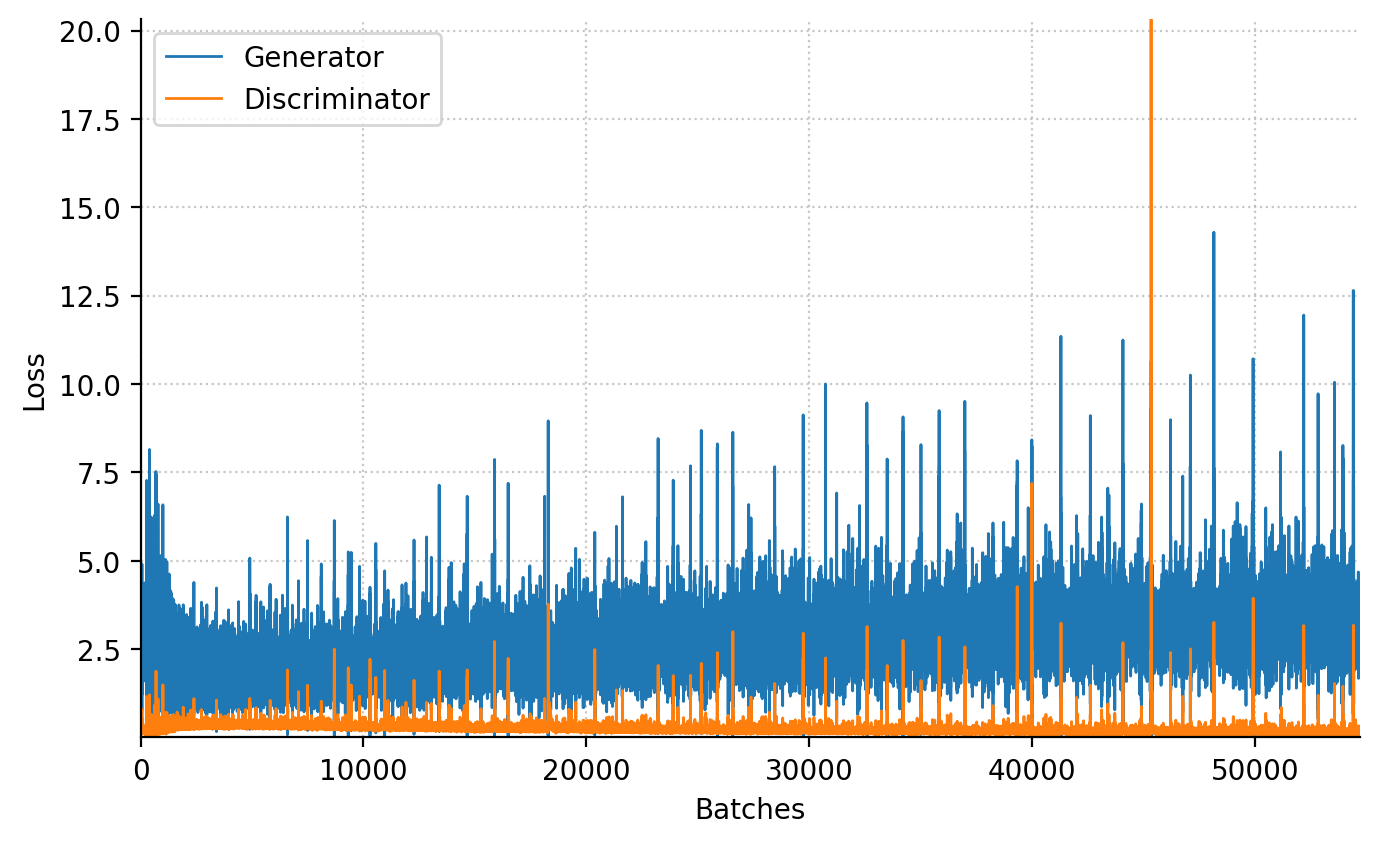
Conclusion

Generative Adversarial Networks (GANs) pair two networks against each other: a Generator that improves its output and a Discriminator that enhances its evaluative skills, converging towards a dynamic equilibrium as training progresses.

In this post, I explore the original GAN, often referred to as the “vanilla” GAN. My goal was to understand the basic mechanics of GANs. Meanwhile, others have advanced this technology, applying it to a range of innovative and fascinating new areas.

• 18 Impressive Applications of Generative Adversarial Networks (GANs)

References

Goodfellow, Ian J., Jean Pouget-Abadie, Mehdi Mirza, et al. 2014. Generative Adversarial Networks. https://arxiv.org/abs/1406.2661.