Research Compute Infrastructure
Our research lab needed a practical way to share CPU, memory, storage, and GPUs among researchers. We built a single-node Kubernetes cluster that allocates those resources through JupyterHub while preserving a familiar notebook workflow. This post describes the original architecture, its design goals, and its availability limitations.
Introduction
Jupyter Notebooks are widely used for interactive computing, programming, and data analysis (Perkel 2018; Mendez et al. 2019; Granger et al. 2021). In our lab, however, personal computers became a bottleneck as projects required more memory, storage, CPU cores, and GPUs. Public cloud services could provide those resources, but their cost model and data-handling constraints did not suit every project. We therefore built an on-premises Kubernetes cluster that lets researchers use shared hardware through a familiar Jupyter environment. This post explains the original architecture, the choices behind it, and the user experience we built on top.
Jupyter Notebooks
A Jupyter Notebook is a JSON-based document composed of cells containing code, prose, equations, and rich outputs (e.g., tables, images, audio, and animations). JupyterLab provides an interface for editing notebooks and running code interactively. Through different kernels, notebooks support languages such as Python, R, Julia, Scala, and C++. Immediate access to intermediate results makes them useful for exploratory analysis, teaching materials, and documented computational workflows.
Because that interactive workflow already suited our research and teaching, we encouraged students and researchers to use notebooks to document and share their work.
Scalability
The notebook interface was not the limiting factor. The problem was running data-intensive experiments on personal computers with limited storage, memory, CPU capacity, or accelerator access. During early research and prototyping, optimizing every workload around those constraints would slow iteration. We considered two broad alternatives: shared HPC infrastructure and cloud services.
HPC systems such as SLING in Slovenia and EuroHPC provide far more compute capacity than our lab could operate. They commonly rely on schedulers such as Slurm, where users describe a job’s resource requirements and submit it to a queue. That batch workflow is appropriate for long or repeatable computations, but it adds friction to the short edit-run-inspect loop we wanted for exploratory notebook work. Interactive HPC sessions can provide a similar experience, but they were not our primary workflow at the time.
Hosted notebook platforms such as Google Colab and Kaggle offer browser-based access to managed compute resources. Their free tiers impose resource and runtime limits. General-purpose providers such as AWS, Azure, Google Cloud, and Alibaba Cloud offer more control, but require cost management and a suitable approach to sensitive data. For our relatively stable workload and hardware budget, operating the equipment locally gave us more direct control over data placement and costs.
An on-premises system trades those concerns for an up-front hardware investment and an ongoing maintenance burden. It does not provide security or lower costs automatically, but it gives the organization direct control over both. That tradeoff made sense for our lab because we already had the hardware and the technical experience to operate it.
The available approaches operate at different levels. Turnkey JupyterHub deployments such as The Littlest JupyterHub focus on the user-facing service. Docker Compose can coordinate a small set of containers on one host. Platforms such as OpenStack manage infrastructure more broadly, while Kubernetes orchestrates containerized workloads across one or more nodes. We chose Kubernetes because its scheduling and resource model matched our goal of allocating shared CPU, memory, and GPUs to isolated user environments.
Kubernetes (often abbreviated as K8s) is an open-source platform for deploying and managing containerized applications. It provides scheduling, resource allocation, health checks, networking abstractions, and mechanisms for scaling workloads. Features such as high availability require a suitable multi-node architecture; Kubernetes alone does not make a single-node deployment highly available.
Docker provides tools for building and running containers, and Docker Compose describes multi-container applications on a Docker host. Kubernetes manages containerized workloads at cluster scope. That additional layer brings scheduling, declarative reconciliation, and service discovery, but also considerably more operational complexity.
We accepted that complexity to retain the familiar Jupyter workflow while sharing the lab’s growing compute capacity.
We designed the system around four requirements:
System scalability: The architecture should allow us to add compute nodes later, although the deployment described here initially used one Kubernetes node.
Resource management: Administrators should be able to define CPU, memory, and GPU allocations for each user environment.
Collaboration: Users should be able to share notebooks and common datasets without giving up isolated working environments.
Interactive access: Users should be able to start work immediately while capacity remains available. Under contention, Kubernetes should share CPU resources and enforce the configured memory and GPU limits rather than maintaining a batch queue.
Architecture
We based the system on Kubernetes to allocate shared resources to JupyterHub user environments (Bussonnier 2018). This section describes the resulting stack and the decisions behind it.
| Service | Solutions (Used in bold) |
|---|---|
| Turnkey solution? | Custom, NVIDIA DeepOps |
| Basic Infrastructure | |
| Operating System | Ubuntu, RHEL, NixOS, Talos |
| Data Storage | ZFS, GlusterFS, Lustre, Ceph, iSCSI |
| System Management | Ansible, Terraform, Puppet, Chef |
| Internal Services | |
| K8s Distribution | upstream (kubeadm), MicroK8s, OpenShift, Rancher |
| Package Deployment | Helm, Kustomize |
| Pod Network | Calico, Canal, Flannel, Weave |
| Storage Provisioner | csi-driver-nfs, Rook, OpenEBS |
| Service Address | MetalLB, cloud-provider integration |
| Ingress Controller | ingress-nginx, Traefik |
| GPU Management | NVIDIA GPU Operator |
| Services for Users | |
| JupyterHub Manager | Z2JH (Zero-to-JupyterHub) |
| Metrics and Monitoring | kube-prometheus-stack, InfluxDB |
Table 1 lists the roles we needed and the alternatives we considered. Bold text marks the selected option. We favored open-source projects with active maintenance, documented bare-metal deployments, and enough adoption to make operational knowledge easy to find. Repository activity and community size informed the decision, but neither served as a single selection metric.
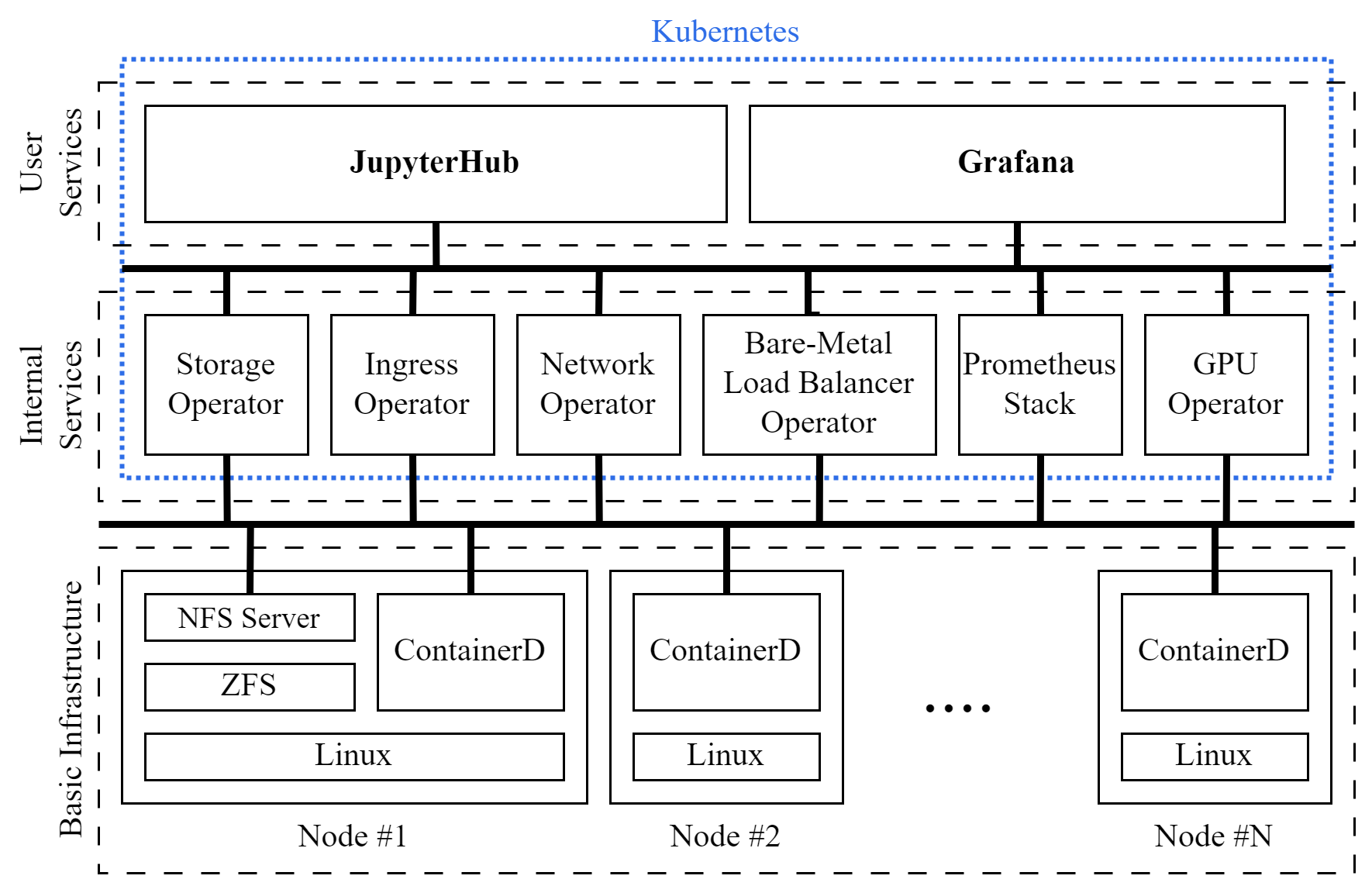
The diagram in Figure 1 separates the system into three levels. The foundation contains the physical node, its operating system, and storage. The middle level contains Kubernetes and the supporting services that users do not access directly. The top level contains JupyterHub and monitoring interfaces exposed to users. Although the design allowed additional compute nodes, the deployment described here ran the control plane and workloads on one physical node.
Turnkey Solution?
We initially evaluated turnkey approaches, including NVIDIA DeepOps. DeepOps combined several relevant tools and offered a supported path, but adopting it still required understanding and adapting its Ansible configuration to our hosts.
Our concern was not that DeepOps removed the need for operational knowledge, but that it added another abstraction to understand during troubleshooting and upgrades. We preferred a smaller stack assembled from components we could inspect directly. This increased our responsibility for integration, but made each dependency explicit.
Foundation Infrastructure
The foundation consisted of the host operating system, container runtime, storage, and configuration management.
Operating system: We chose Ubuntu Server, a Debian-based Linux distribution with extensive documentation and broad support from the projects in our stack. We also considered RHEL-based distributions, the declarative NixOS, and the Kubernetes-focused Talos. Ubuntu was the option our team knew best, which reduced operational risk.
Container runtime: We selected containerd, an open-source container runtime that implements Kubernetes’ Container Runtime Interface (CRI) and is supported by NVIDIA’s tooling.
Data storage: We chose OpenZFS for storage on the cluster node. Distributed systems such as GlusterFS, Lustre, and Ceph can spread data and failure domains across hosts, but they require additional infrastructure and operational work. ZFS gave us snapshots, compression, copy-on-write semantics, block checksums, and RAID-Z redundancy within one server. Checksums allow ZFS to detect corrupted blocks, and redundancy allows it to repair them during reads or scrubs. The tradeoff was a clear single point of failure: ZFS did not distribute our pool across Kubernetes nodes. OpenZFS dRAID does not change that property. It distributes parity and spare capacity across disks within a ZFS vdev to accelerate recovery after a disk failure, not across independent storage hosts (OpenZFS documentation). At the time of this deployment, an existing RAID-Z vdev could not be widened one disk at a time. OpenZFS 2.3 later added RAID-Z expansion, which supports attaching a new disk to an existing RAID-Z vdev without changing its parity level (OpenZFS documentation). It therefore cannot convert RAID-Z1 to RAID-Z2. That migration still requires creating a new RAID-Z2 pool and copying or restoring the data.
We exported the ZFS datasets over NFS and mounted them through Kubernetes. NFS supports ReadWriteMany volumes, allowing pods on multiple nodes to mount the same volume when the server export permits it (Kubernetes documentation).
System management: We used Ansible for remote configuration because we already had positive experience with it and could keep the host setup in version-controlled playbooks.
Kubernetes
Kubernetes provides core abstractions for scheduling workloads, exposing services, and allocating CPU and memory. Cluster add-ons and operators supply capabilities such as pod networking, persistent storage, ingress traffic management, monitoring, and GPU discovery.
Some add-ons use the operator pattern: a controller watches Kubernetes resources and reconciles the actual state toward the declared state. Not every add-on is an operator, but the same reconciliation model appears throughout the platform.
An operator often introduces custom resources that describe application-specific state. Its controller then creates or updates lower-level Kubernetes resources and reacts when the observed state changes.
Internal Services
The following components were not exposed directly to users, but supplied networking, storage, ingress, and accelerator support for their workloads.
Kubernetes distribution: We examined Canonical MicroK8s, Red Hat OpenShift, and an upstream installation managed with kubeadm. We chose the upstream route because it let us select and configure each cluster add-on ourselves.
MicroK8s offered a compact installation and convenient add-ons, but its Snap-based packaging and bundled conventions differed from how we wanted to manage host configuration and external NFS storage.
We ruled out OpenShift because adapting every service to its security model would have added work that our small, trusted-user environment did not justify.
Package deployment: Kubernetes resources can be declared directly in YAML manifests. Larger applications often distribute those manifests as configurable packages. We used Helm, which renders parameterized templates and manages each installed package as a release.
Pod networking: Kubernetes requires a Container Network Interface (CNI) implementation so pods can communicate. We selected Tigera Calico, which provided the routing and network-policy support we needed.
We also considered Flannel, a narrower networking component. Calico’s network-policy support and range of routing options made it a better fit for a cluster we expected to extend over time.
Persistent storage: We used csi-driver-nfs to provision Kubernetes PersistentVolumes on our existing NFS export.
Centralized storage simplified backups and troubleshooting, but every workload still depended on the node hosting NFS. The CSI driver automated volume provisioning; it did not remove that availability limitation.
Bare-metal service address: Public-cloud Kubernetes integrations can allocate external IP addresses for LoadBalancer services. Our bare-metal cluster had no such integration, so we used MetalLB to allocate an address from our local pool and announce it to the network. On this single-node deployment, MetalLB made the service reachable but could not provide node-level load balancing or failover.
Ingress controller: The ingress controller accepted HTTP and HTTPS traffic from outside the cluster and routed requests to Kubernetes Services according to host and path rules declared in Ingress resources. DNS remained external to Kubernetes and pointed the public hostname at MetalLB’s address. This kept ephemeral pod addresses out of the public configuration and allowed traffic to be distributed among replicas of a service.
We considered ingress-nginx and Traefik. Both implemented the Kubernetes Ingress API, but differed in configuration, extensions, and operational behavior. We selected ingress-nginx at the time.
GPU Operator: We used NVIDIA’s GPU Operator to install and manage the components that expose GPUs to Kubernetes workloads. We initially kept the NVIDIA driver on the host so the GPUs would remain usable outside Kubernetes. Driver-version conflicts made that arrangement difficult to maintain, so we moved to the operator-managed driver containers.
User Services
Users interacted primarily with JupyterHub and a read-only Grafana dashboard.
JupyterHub provided authenticated access to compute resources, data, and notebooks. We deployed it with the Zero to JupyterHub Helm chart.
After authentication, each user received an isolated container without administrative privileges. Kubernetes attached the user’s persistent storage and shared directories, and assigned a GPU when the selected profile requested one and capacity was available.
JupyterLab started automatically inside the container and included a Linux terminal. Users could install additional packages with pip, conda, or mamba.
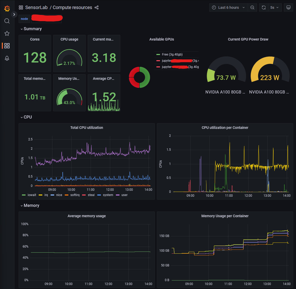
Grafana displayed the cluster’s current workload and GPU availability so users could decide when to start resource-intensive work. The kube-prometheus-stack chart deployed Prometheus for metric collection and Grafana for visualization.
Deployment
This section summarizes the hardware and the resulting user experience.
Hardware
| Hardware | Specifications |
|---|---|
| Chassis | Supermicro A+ Server 4124GS-TNR, 4U, up to 8 PCIe GPUs |
| CPU | 2x AMD EPYC 75F3 (32C/64T, up to 4.0 GHz, 256 MB L3 cache) |
| Memory | 1 TB (16x64 GB) registered ECC DDR4, 3200 MHz |
| System | 2x 2 TB NVMe SSD, software RAID-1 mirror |
| Storage | 6x 8 TB SATA SSD, ZFS RAID-Z1 (one-disk redundancy) |
| GPU | 2x NVIDIA A100 80 GB PCIe |
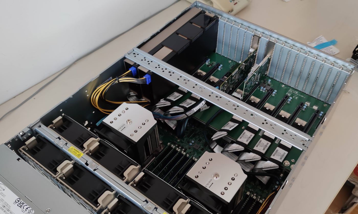
When we bought the hardware in early 2022, we chose third-generation AMD EPYC processors. The F-series traded some core count for higher base and boost frequencies, up to 4.0 GHz in this model. We selected the 280 W EPYC 75F3 and populated all eight memory channels on both processors with sixteen registered ECC DIMMs. In our evaluation, this AMD configuration offered a better price-to-performance ratio than the Intel alternatives we considered.
One concern was the behavior of Intel-optimized numerical libraries on AMD processors. Older Intel MKL releases could select a slower code path on non-Intel CPUs unless configured otherwise (discussion and measurements). OpenBLAS provided an alternative, and conda-forge’s nomkl package made it possible to prefer that stack in Conda environments.
We mirrored two NVMe drives for the system volume and configured six 8 TB SATA SSDs as a ZFS RAID-Z1 data pool, which can tolerate one drive failure. Two NVIDIA A100 GPUs supplied accelerator capacity.
NVIDIA A100 GPUs were available as PCIe cards or SXM4 modules. SXM4 offered a higher power envelope and high-bandwidth GPU interconnects through NVSwitch, but required a compatible baseboard. PCIe cards had a lower power limit and more restricted NVLink topology, but fit a conventional server platform. We chose PCIe to retain more flexibility when replacing or mixing accelerators later.
We expected most data transfer to occur between CPU memory and a single GPU instance. Multi-Instance GPU (MIG) mode let us partition each A100 into isolated instances for independent users. Changing the partition layout required recreating those MIG instances.
User Experience
After deploying the hardware and software stack, we ran a month-long stabilization period. We warned users that the system could be rebooted or reconfigured and that they should keep independent copies of important data.
We made two different resource-allocation choices. CPU remained oversubscribed, so users could request work immediately and the Linux scheduler shared CPU time under contention. Memory was not safely compressible in the same way: when the node ran out, Linux could terminate a process selected by its out-of-memory scoring. This made memory exhaustion less predictable than ordinary CPU contention and was a limitation of the permissive policy.
Informal feedback from students and researchers was positive. They particularly noticed the additional CPU cores, memory, and access to isolated GPU instances.
The test period also exposed missing workflow features. In response, we added shared directories for datasets and notebooks, a shared package cache, and better persistence for tasks launched from JupyterLab.
JupyterHub
JupyterHub required little user training because students and researchers were already familiar with JupyterLab. The main change was that their environment now ran on shared cluster hardware rather than a personal computer.
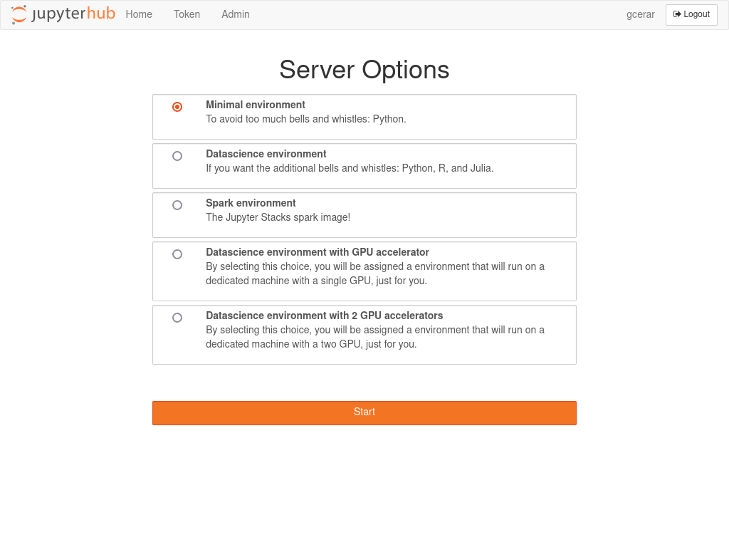
Upon logging into JupyterHub, users selected from predefined container profiles, as shown in Figure 3:
- A minimal working environment.
- A comprehensive data science environment equipped with multiple packages and support for Python, R, and Julia.
- A selection of containers offering GPU instances.
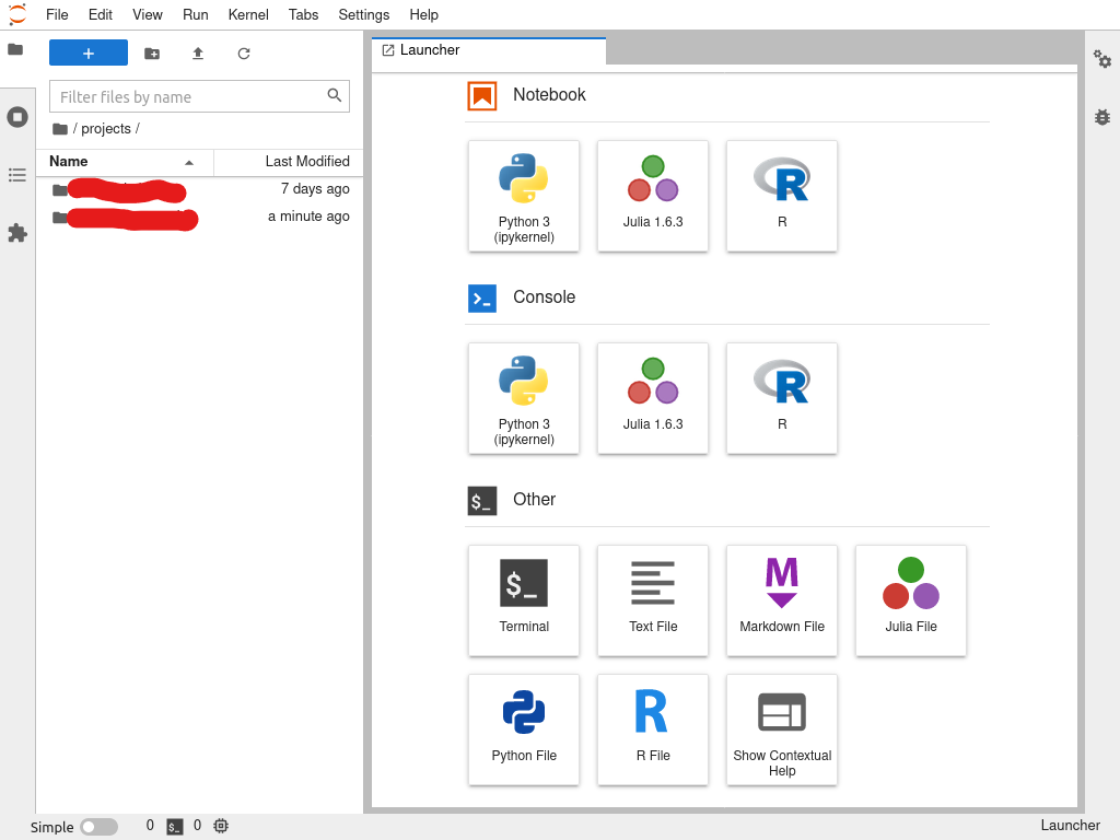
The development environment presented a layout similar to modern IDEs, with a file explorer on the left and editor tabs on the right (see Figure 4).
Grafana
Users had read-only access to a Grafana dashboard showing total and per-container CPU use, memory use, GPU utilization, temperatures, and storage I/O (see Figure 5).
Conclusions
This project moved our lab’s notebook workflow from personal computers to a shared Kubernetes node. JupyterHub preserved the interactive environment users already knew, while Kubernetes isolated their containers and allocated shared CPU, memory, storage, and GPUs.
The architecture could accommodate additional compute nodes, but the deployment described here was not highly available. Its control plane, workloads, and ZFS-backed NFS storage all depended on one physical server. Kubernetes simplified workload management within that boundary; it did not remove the server as a failure domain.
The central engineering tradeoff was operational complexity. Kubernetes and its add-ons gave us consistent resource allocation, persistent user environments, and room to expand the cluster, but each additional component also created another upgrade and compatibility responsibility.
At the time, the next step was to use Prometheus data to measure resource contention and refine the allocation policy. In hindsight, lifecycle management deserved equal priority. The architecture worked, but its value depended on keeping the control plane and every critical add-on within supported upgrade paths.
Three years later, neglected upgrades caught up with this infrastructure. See Research Compute Infrastructure, Revisited for the migration that followed.